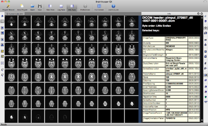
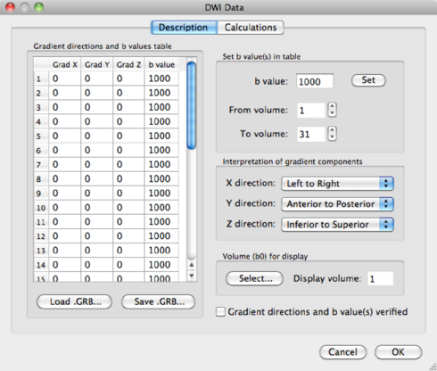
The DMR project just created may look like this, where the first volume is displayed. In this case, it is the b0 volume. This volume contains 75 slices.
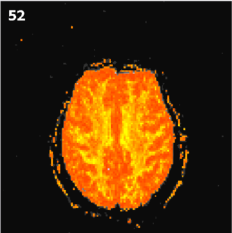
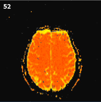
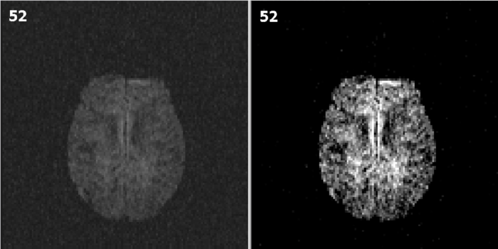
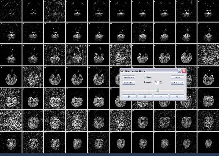
You may explore the data via Options --> Time Course Movie. By clicking the play buttons >, BV will move through the volumes or diffusion directions of your measurement. The Recalibrate button in the Time Course Movie window automatically adapts brightness to the slice you are currently viewing. This feature is added because the intensities of a b0 images are far higher than those of a DW image.
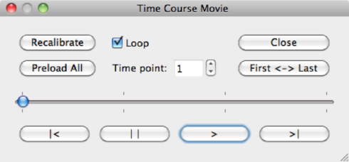
| Recalibrate | Recalibrate the intensities of the current volume |
| Preload all | Load all volumes in memory (on slower machines) |
| Time Point | Enter a value here to go directly to a specific volume |
| Loop | When checked, BV will loop the volumes |
| First <-> Last | Switch quickly between the first and the last volume of the data set |
The slice before and after recalibrating are shown below:
On the basis of the DMR data, it is possible to directly calculate tensors, FA and Mean Diffusivity maps. For background on tensor estimation, see [?, ?] among others. To recap, Mean Diffusivity is defined as
 | (1.1) |
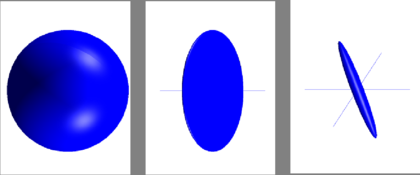
and is in theory limited to the interval [0, ∞). Fractional Anisotropy is defined as
 | (1.2) |
Fully isotropic voxels have FA = 0, while fully anisotropic voxels have FA = 1. This is illustrated in figure 1.1.
Let’s continue with the FA calculation procedure in BrainVoyager:
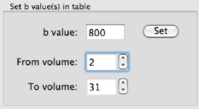
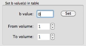
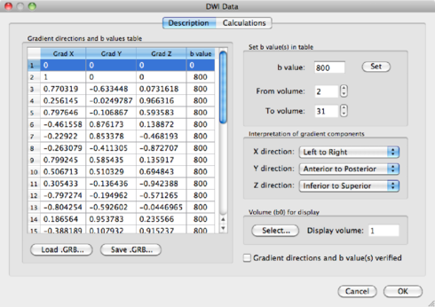
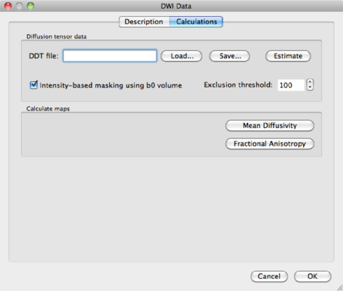
You have the option here to mask out the background of the image. Please bear in mind that, by masking via a threshold, you always risk losing voxels in the brain itself. It is safer to use a mask based on the anatomical data, which is discussed in section 1.6.3. For now, because of the nice visualisation, check the mask box and click on Estimate to start the tensor estimation. After the calculations, BV will ask you to save the resulting DDT file, containing the tensor information. Save it as human31dir_dmr.ddt. The ddt calculated from a dmr is different from the ddt calculated from a VDW file.
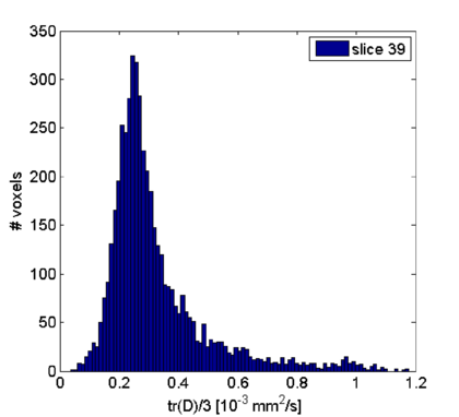
In principle, one could start a complete analysis on these maps. For instance, to create a MD histogram of slice 39 (done in Matlab):
The disadvantage is that we stay in 2-D space. To do an analyis in 3-D, the DMR project has to be co-registered to a VMR, which is explained in the next sections.