1.6 Tensor, Diffusivity and FA calculation

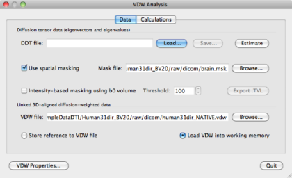
First, close the VMR you may still have open, and reopen it (beware to use the _ACPC.vmr or _TAL.vmr if you went into standard space). Go to DTI --> Diffusion Weighted Data Analysis. A VDW Analysis window appears. In the Linked 3-D aligned diffusion weighted data part, click the
Browse button and point to the VDW file created in the previous part, which is human31dir.vdw.

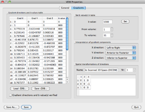
Next, go to VDW Properties in the VDW Analysis window. You’ll find the gradient table on the left and some other info on the right.

1.6.1 The gradient table

The gradient table can be filled in two ways: manually, by entering the gradient direction and b-value directly into the table, and automatically by loading a so-called GRB GRadient and B-value file.

You might have a text file with gradient directions or otherwise you have to ask your MR technician for such a file.

For this particular experiment, we need a gradient table with 31 directions. If the gradients are not yet specified, do it by clicking "Load .GRB” and locate the file mgh_dti30.grb. The gradient table can also be found in appendix ??.

Now that the gradient table is filled, click the Gradient directions and
b-values verified check box, and the VDW file can be saved by using Save As or Save. BV will remember the associated GRB file. The Set b-value(s) in table option on the top right may be used for changing the b-value as well, for bulk changes. You need to set correct b-values for your experiment, which in this case are: measurement 1: b=0, measurement 2-31: b=800. Typing directly in the table is also supported.

The interpretation of gradient components part of the VDW
Properties window may be used if the data is flipped/reversed. The Spatial transformations of directions part may be used if BV makes a wrong interpretation of the scanner versus subject coordinate systems. Both options are explained in Appendix 3.1.1.

Press OK to leave the VDW Properties window. You will return to the VDW Analysis window.

1.6.2 Tensor, Mean Diffusivity and FA Computation

Once the VDW file and gradient information are correct, click Estimate in the VDW Analysis window. Warning: BV may look irresponsive, but in fact it is busy calculating tensors. A DDT “Diffusion Tensor” file is created, and BV asks you to save this file. Save it as human31dir_vdw.dmr. A DDT file may also be saved in TVL format, by clicking the Export TVL, for use in the TrackMark software (information via support@brainvoyager.com).

1.6.3 Recommended: masking the DDT data

In general you are not interested in data outside of the brain. Due to the nature of the acquisition however, there is noise present outside of the brain, which should be masked out. Besides the visual attractiveness, this also reduces the amount of voxels significantly, which increases processing speed in later steps. The pipeline for mask creation is as follows:

VMR → Peel brain → VOI containing the brain → Mask file → apply mask file to VDW

We have already created a VMR containing only brain tissue. Open it and link the VDW file created in section 1.5 to the VMR: DTI -> Diffusion Weighted Data Analysis. In the Linked 3D-aligned diffusion-weighted data section, locate the VDW that was created earlier using the Browse button.

Now it’s time to define a VOI containing all brain voxels. In order to get a smooth VOI without any holes in it, click the Gaussian button in the segmentation tab.

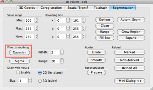
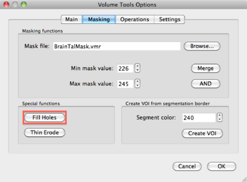
Go to the 3D Volume tools -> Segmentation. Set Value range: Min to 1 and Value range: Max to 225, and hit the Range button. All brain voxels should be selected now and displayed as blue voxels. Now it’s time to fill any holes which might still be present in the mask. Go to 3D Volume tools -> Segmentation -> Options -> Masking, and click the Fill Holes button, and then OK.

At first, it seems like nothing has happened, but if you click inside a blue region, the screen will be updated and holes will have disappeared.

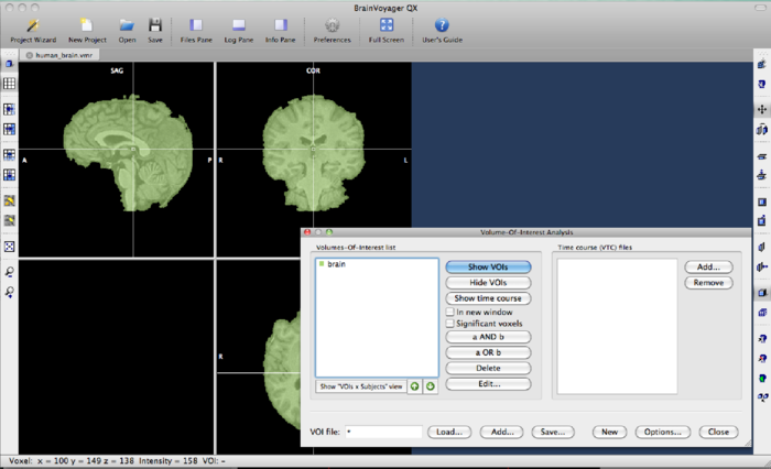
Now, go to 3D Volume tools -> Segmentation -> Options -> Define VOI. A dialog pops up and give brain as the name of the VOI. Save the VOI using the Save button. The BrainVoyager window should look like this:

The VOI can now be converted to a mask file. Go to Analysis->Region-Of-Interest Analysis. A dialog will open with the VOI “brain” in it. Save the VOI by clicking the Select this VOI by clicking on it, and hit the Options button. In the VOI functions tab, set the options as follows:

and save the mask file as brain.msk.

To apply the mask to tensor calculations creation, re-open the file human_brain.vmr. Go to DTI -> Diffusion Weighted Data Analysis. Load the VDW created in section 1.5. Then, tick the use mask checkbox, and locate the mask file brain.msk with the Browse button:

Hit the Estimate button to create a masked DDT file and save it accordingly as human31dir_vdw_masked.ddt.

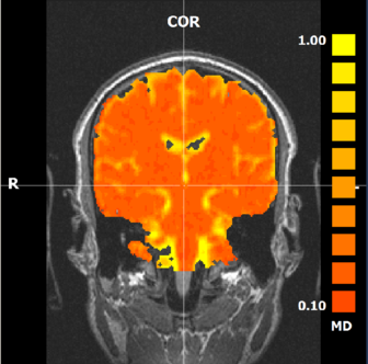
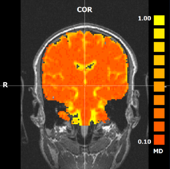
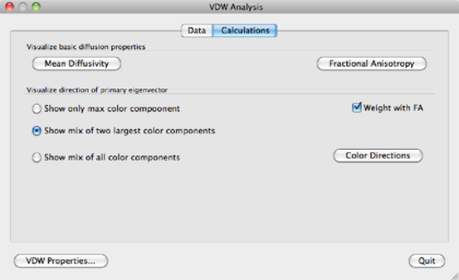
FA and mean diffusivity can be calculated in the Calculations tab in the VDW Analysis window.

Mean Diffusivity is defined as

(1.3)

and is in theory limited to the interval [0, ∞). Click the Mean Diffusivity button to produce a MD map, overlayed on the VMR. Upon clicking this button, a map, interpolated to VMR resolution is created. However, in most cases one would like to see the map in DWI resolution. This can be established via Analysis --> Overlay Volume Maps and un-checking the interpolate checkbox. Also in this window the value range can be set.

(a) MD in VMR resolution (interpolated)

(b) MD in DWI resolution

Figure 1.4: Mean Diffusivities

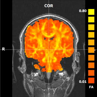
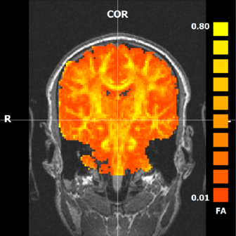
Fractional Anisotropy is defined as

(1.4)

Fully isotropic voxels have FA = 0, while fully anisotropic voxels have FA = 1. Click the Fractional Anisotropy button to calculate a FA map overlayed on the VMR. Again this map is in VMR resolution.

For users of BrainVoyager 1.10 or lower: Be careful! For visualisation purposes, FA is scaled up a factor 10 in BrainVoyagerQX < 1.10!. So, FA = 2.0 in the map is in reality FA = 0.2.

(a) FA in VMR resolution (interpolated)

(b) FA in DWI resolution

In both MD and FA maps, values may be explored by moving the mouse pointer around. Values, reported as t=0.32781, are displayed in the Log tab of the Sidebar, or in the status bar in the lower left of the screen.

1.6.4 Alternative Diffusion Measures

Of course we can extract the values of the eigenvectors and compute alternative diffusion measures such as shape measures, radial/axial diffusivities, trace(D) from the tensor file. This is implemented in a Matlab function available on http://support.brainvoyager.com/diffusion-weighted-imaging/66/349.

1.6.5 Color coded maps

Color coded maps can be displayed by selecting one of the options in the Visualize direction of primary eigenvector part of the VDW analysis window. It is initially recommended to choose the Weight by FA option, see figure 1.5(d). The color options are:

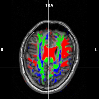
(c) FA map based on 3 max components

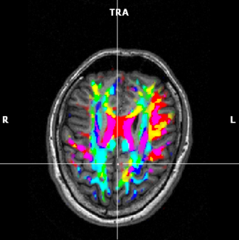
(d) FA map based on a mix of 2 max components

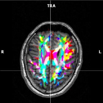
(e) FA map based on a mix of 3 components

(f) FA map based on 2 components, but not weighted by FA, showing all data.

Figure 1.5: Color options for a FA or MD map, shown for a FA map.

In figure 1.5 the different options are shown. The transparency of the colors may be changed using the Ctrl+Arrow up/down key combination.