We will now start by preparing the anatomical data. The anatomy is used to transfer the data into a common space (Talairach space, abbreviated as TAL). The transformation files are later on used to transfer the DW-MRI data into TAL space as well.
It is assumed that you know how to put an anatomical data set into TAL space. If not, please go through the BVQX Getting Started Guide.
For each subject, create the <subject>_TAL.vmr file. Make sure you do not delete <subject>_ACPC.trf and <subject>.TAL.
For each subject in your study, do the DW-MRI data analysis in native space, up to the point of creation of FA and ADC maps. Save each map as <subject>_FA.vmp or <subject>_ADC.vmp respectively.
The processing of FA maps is demonstrated here, but it is the same for ADC maps. It consists of two steps: 1) bringing the map to ACPC space and 2) going from ACPC to TAL space.
Map to ACPC space Open the native space VMR, <subject1>.vmr. Go to Analysis -> Overlay Volume Maps. Click Load VMP and load the file <subject1>_FA.vmp you have created earlier. Close the dialog. You should see a FA map overlayed on anatomy.
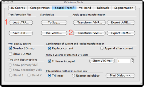
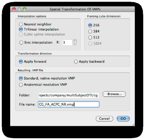
Now, go to 3D Volume Tools -> Spatial Tranf. Load the <subject>_ACPC.trf file created earlier and click Transform .VMP.
Save the result as <subject>_FA_ACPC.vmp:
The ACPC transformation is done. Close the VMR.
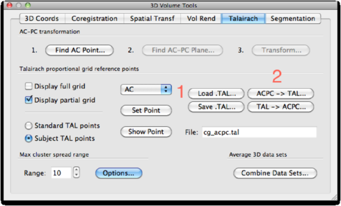
Map to TAL space from ACPC Now, open the file <subject>_ACPC.vmr. Load the FA map: <subject>_FA_ACPC.vmp. Go to 3D Volume Tools -> Talairach. Load the TAL file <subject>_ACPC.TAL by clicking the Load TAL button. Next, click ACPC -> TAL.
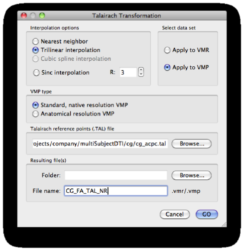
Save the results as <subject>_FA_TAL.vmp (make sure the Apply to VMP checkbox is checked!):
Repeat the talairach process for each subject.
Now that we have created FA maps in TAL space, and have reframed them for each subject, it’s time to do simple statistics. For analysis, first a TAL VMR needs to be opened. You may use the best VMR in your data set, but you can also create an average VMR from all data sets (Volumes > Combine 3D data sets).
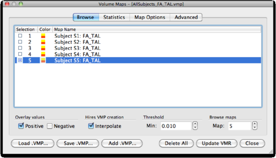
Open the Analysis > Overlay Volume Maps dialog. This dialog can also be opened using the Ctrl+M shortcut. Now, load the FA map of each subject:
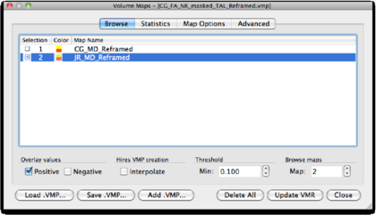
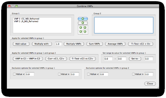
Browse all maps to see whether they correctly align with the VMR and inspect for other irregularities. Now we can use the Combine VMPs option in the Advanced tab. The dialog is divided into 4 parts. The top part shows the subjects maps, and gives you the opportunity to discriminate between 2 groups G1 and G2. A second part that can be used to analyze the maps without splitting them into groups. A third part that enables specific statistics on the basis of the maps separated into groups. Finally, an ”exclusion” option that will help to shape specific maps according to their values and a value range selected by the user.
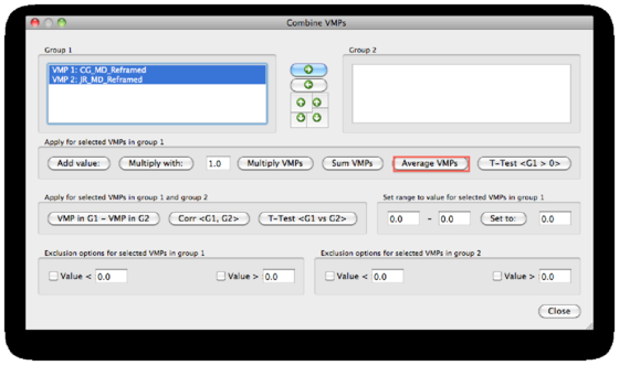
First, we try the statistics that are available for the single group (in the first field). We mark all subjects maps and use the Average VMPs option.
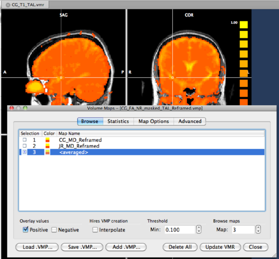
As the result, a new map will be created in the main dialog (at the end of the map list). We check the map to visualize the result of the average procedure.
For this step, first create a map containing all maps (VMPs) of all subjects, and use the naming convention Subject <initials>: FA or the like:
Then, go to the Advanced tab of the Volume Maps dialog. From there on, you can use the ANCOVA tool just as you would for an fMRI ANCOVA analysis. I’d like to refer you to the description in the User’s Guide in the Basic Analysis, Random Effects Group Analysis section. You can also have a look at the description in http://web.mac.com/rainergoebel/RainersBVBlog/Rainers_BV_Blog/Entries/2007/9/25_The_'C'_in_ANCOVA.html.
As an example, I’ve divided 5 subjects into two groups (Dummy example, i.e. excellent readers in group 1 and poor readers in group 2), and I’ve added age as a covariate. The design table of the experiment looks like this:
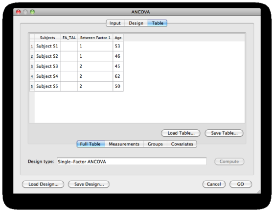
Click GO to start the analysis.