Brain Innovation

Analysis: Fixed Effects

This guide uses the ClockTask experiment as an example, which is described over here.

Close any open projects. Open the "BS_TAL.vmr" project file located in the ClockTask folder and then select the General Linear Model: Multi study item in the Analysis menu. This will invoke a dialog titled General Linear Model: Multi Study, Multi Subject.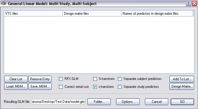


The large central region of the dialog shows the multi study list box which is empty when you invoke the dialog. When filled, each row of this list box will refer to a single study (VTC file name) together with an associated single-study design matrix (RTC file name). The multi study list box is filled sequentially with pairs of single-study data and design matrix files. In this example, we will include four studies, two runs from two subjects. Click the Add to List button to specify the necessary files for the first study. 

The appearing Open dialog asks for a VTC file. Select the file "BS_run1_r1_pp.vtc" which contains the data of the first run of the first subject and click the Open button. A second Open dialog appears asking for a single study design matrix (SDM/RTC) file. Select the file "ClockTaskDesignMatrix_run1.rtc" and click the Open button. The first row of the multi study list box will now be filled as shown below: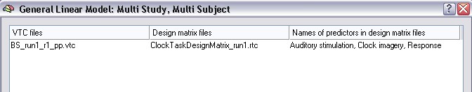 


So, the first column of the first row now refers to the VTC data file to be included in the multi study GLM. The second column contains the single study design matrix filename (RTC) specifying the statistical model to be used for the data file in the first column. The last column shows the names of the predictors found in the RTC file. The predictor names are shown so that you can check that each subsequently included study (RTC) uses the same predictors in the same order. 

Note: Each included study must use the same predictors defined in the same order so that the program can combine predictors with the same "meaning" (i.e. equal conditions) across studies. The defined time course of corresponding single study predictors (condition Auditory stimulation in study 1, condition Auditory stimulation in study 2, etc.) can be, however, different for each study; this allows, for example, to present individual trials in randomized order and/or to balance the order of trials across runs and/or subjects. In the example experiment, the time points and the order of the trials in the different runs were identical, thus, we can use the same single study design matrix file for all runs/subjects. More generally, however, you might want to use a different design matrix file for each single run.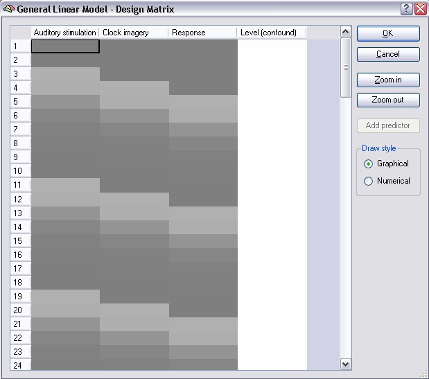

As with single studies, we can check at any time the current state of the internally built design matrix. Simply click the Design Matrix button in the right lower part of the dialog to invoke the design matrix display dialog. 

In the design matrix display, time runs from top to bottom, whereas in the Single Study General Linear Model dialog, time runs from left to right. Each column represents one predictor. The first column contains a graphical representation of the defined predictors with its names, e.g. Auditory stimulation, shown in the column header. In this representation, numerical values within a cell are shown as grey levels: a value of 1.0 is colored white, a value of -1.0 is colored black and each intermediate value is colored with the respective shade of grey. The numerical values are made visible by clicking on the Numerical button on the right. 

These values are the results of the convolution of the box car function with the hemodynamic response function. If you visualize the design matrix prior to pressing the HRF button, you would see only 1.0 and 0.0 values in the first three columns. The fourth predictor with a constant value of "1" (entirely white) has been added automatically to the design matrix and is necessary for the GLM to estimate the level of the fMRI signal at each voxel. Such a constant predictor will be added automatically for each study. You can use the scroll bar(s) to browse to any position within the design matrix or you can zoom in and out. You can also increase the size of the dialog by using the size grip in the right lower corner. 

Note: The design matrix is used exactly as shown in this dialog for the subsequent GLM computation. In order to know precisely what statistical model is constructed and used by BrainVoyager, you can always check the design matrix in this dialog. In addition, the actually used design matrix is also saved to disk automatically at the beginning of a GLM computation ("DesignMatrix.txt"). It can thus be used easily in external calculations, e.g. computing the intercorrelations between predictors using Microsoft Excel. 

The design matrix looks exactly identical to the one we have created interactively in the Single Study General Linear Model dialog. This is, of course, to be expected since we have included just one study so far and specified the design matrix file we have saved previously. If we would run the multi study GLM right now, it would, thus, compute exactly the same result as the single study GLM. 

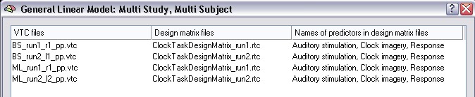
Click the Cancel button to close the design matrix dialog. We now add three more studies by clicking the Add button three more times, every time specifying another VTC file / RTC file pair. So, we add the VTC file for run 2 of subject "BS" with the respective design matrix file. Then we add the files for runs 1 and 2 of subject "ML". There also exist files for run 3 and 4 in the "ClockTask" folder, but we will not use these files here. The dialog should now look as shown in the figure below: 

Let's now inspect the internally built multi study design matrix again by clicking the Design Matrix button. After clicking the Zoom out button several times, the design matrix should look as shown in the following figure:

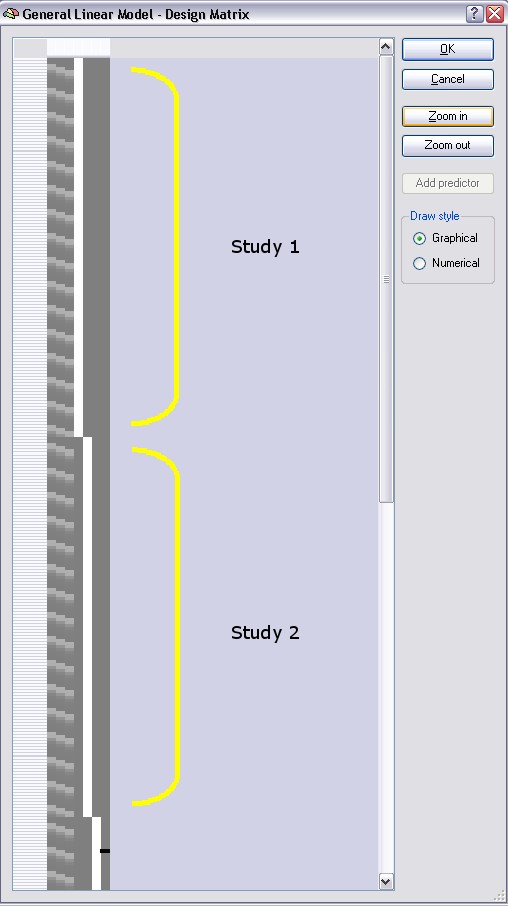
The three main predictors are shown in the first three columns as before, however they extend now over all four runs. In other words, the multi study design matrix has been created by concatenating the four single study design matrices. We have, thus, one set of predictors across all studies. This is one of three ways how the program constructs a multi study design matrix, the other two ways using separate sets of predictors for each study or subject will be described shortly. In the figure above the design matrix segments for the first two studies have been labeled with yellow brackets ("Study 1" and "Study 2"), the time points of the third study are only partially visible and the fourth study is not visible in the figure. You can, however, browse with the vertical scroll bar to any section of the design matrix. 

Note that BrainVoyager has added four signal level "confound" predictors automatically. Each of these predictors is set to a value of 1.0 (white color) for all time points of a study and to 0.0 (grey color) for the remaining studies.

Note: The different constant terms for the different studies allow each study to have a different signal level. This is very important since often different runs of different subjects - and sometimes even runs of the same subject in the same scanning session - produce different signal levels. A visualization of these study level effects can be obtained for any region-of-interest with the ROI GLM analysis tool. If you check the z-transform option in the General Linear Model: Multi Study, Multi Subject dialog, the signal level confounds will be estimated as 0.0 because the mean of the signal time courses will become zero after the transformation. In this case, the study signal level confounds could be removed from the design matrix (but they remain included in the present version of BrainVoyager, for one to get the correct number for the degrees of freedom). If you uncheck the z-transform option, each study constant predictor will be estimated as the mean of the data points belonging to the respective study.

The concatenation of the predictors means that the signal changes at a voxel time course are estimated by the same three values (beta weights of the three main predictors) across the concatenated data points. This is also reflected in the resulting GLM where you will find the three main predictors for specifying contrasts. To check this, close the design matrix dialog and run the GLM by clicking the GO button. If you then invoke the Overlay General Linear Model dialog, it will look as below: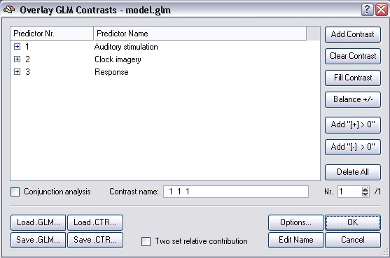

The three filled rows represent the three main predictors of the multi study design matrix. You can now specify contrasts and compute statistical maps showing voxels where a contrast reaches significance across the four studies. 

The concatenation approach to build a multi study design matrix is a reasonable approach if the included studies are multiple runs of the same subject. If runs from multiple subjects are used, the results will not reach highly significant levels at non-aligned brain regions. Using spatial smoothing, the likelihood to have corresponding active regions across subjects can be increased (however this approach has other problems which are not discussed here).

• Prev
• Next