Brain Innovation

Extraction of Beta Values

BVQX version used: 1.9.10
Dataset: 5 Subjects dataset, BV QX advanced exercises

1. 1. First, we run a RFX GLM.

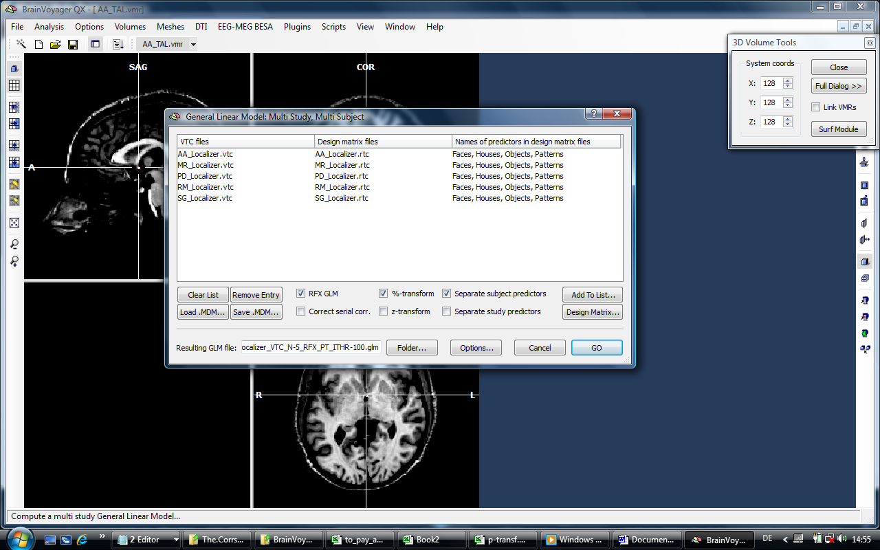
We use the % transformation to normalize the time-courses.

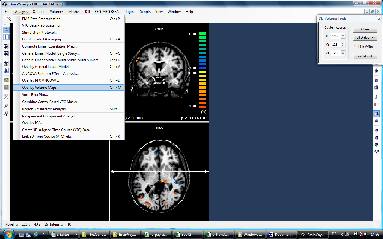
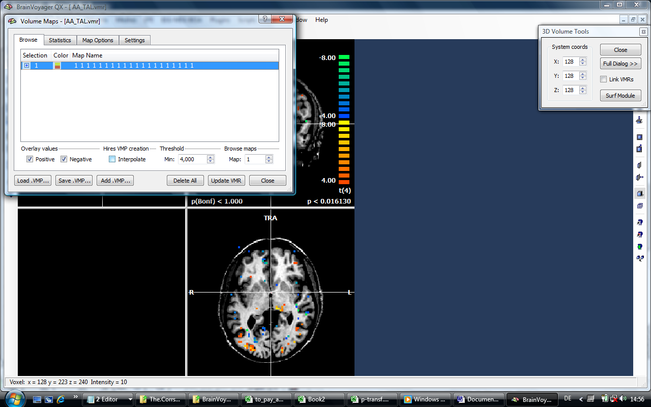
2. 2. In the “Overlay Volume Maps” dialog, we check off the interpolation of the statistical map.

3. 3. In the “Talairach” tab of the 3D volume tools, we check a size of 3 (in each axis) to enable a coverage of 27 (anatomical) voxels in total.

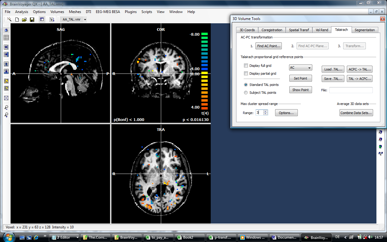
4. 4. We select an area on the left side of the dataset. Due to the selection set before, we just select 18 voxels who have exactly the same statistical parameters (so they cover the same functional voxel). Alternatively, on could set the spread range to “1”.

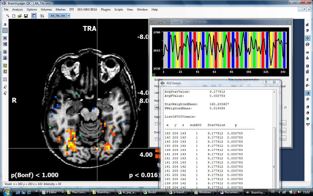
In this case, the clusters covers 18 (anatomical, 1mm) voxels.

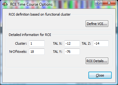
5. 5. We define a Volume of Interest file (VOI) based on the cluster selected.

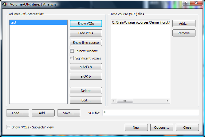
6. 6. We open the Options of the VOI Analysis tool.

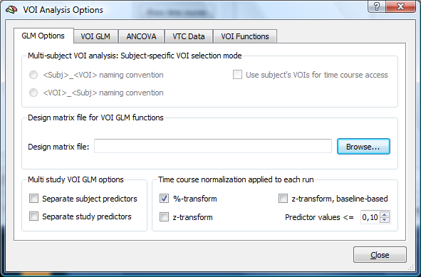
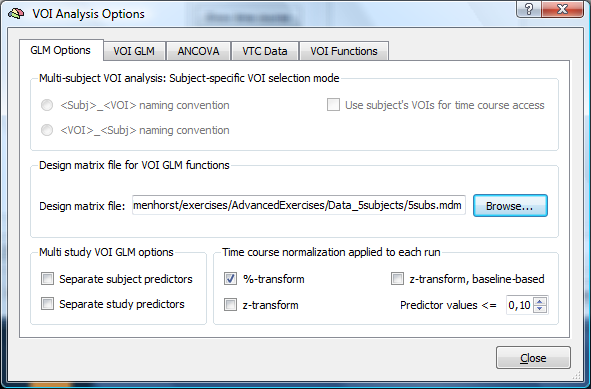
7. 7. We load the MDM file used to run the previous RFX GLM analysis.

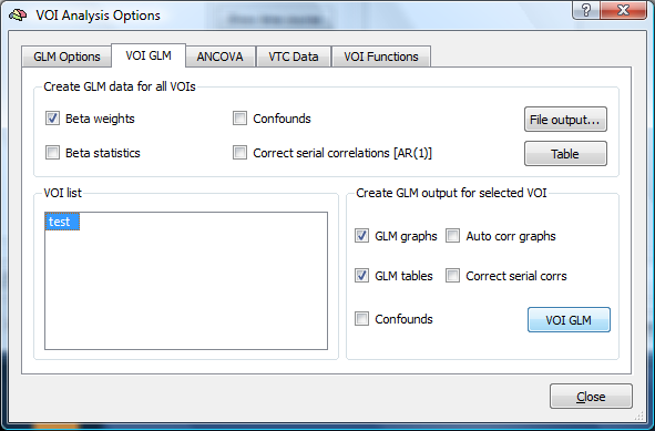
8. 8. We switch to the “VOI GLM” tab and click the “VOI GLM” button.

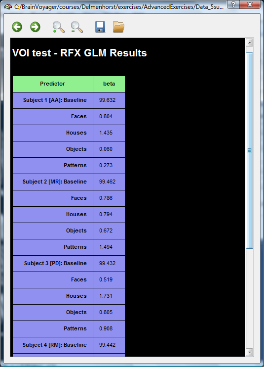
9. 9. In the ROI GLM specifications, we check the “Separate subject predictors” and RFX GLM checkmark.

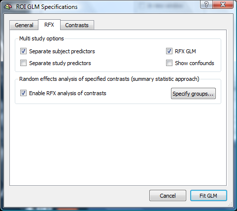
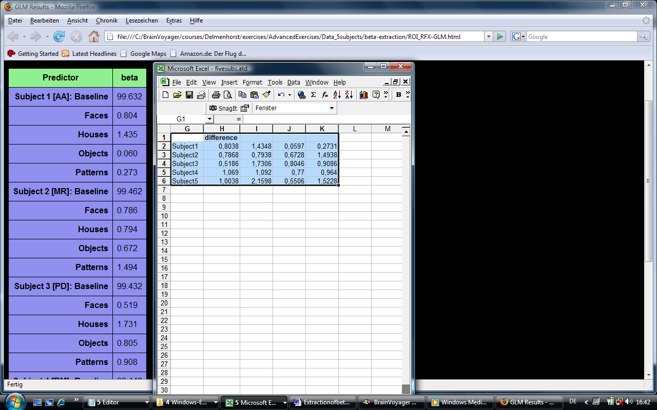
We obtain an HTML table containing beta values separated by subjects and conditions.

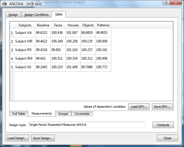
10. 10. We perform a different operation to extract the betas. This time, we select the Ancova tab in the options of the ROI Analysis tool.

11. 11. We load the same MDM file (using the same time course normalisation), and click the button called “Extract values” to obtain a table with the betas.

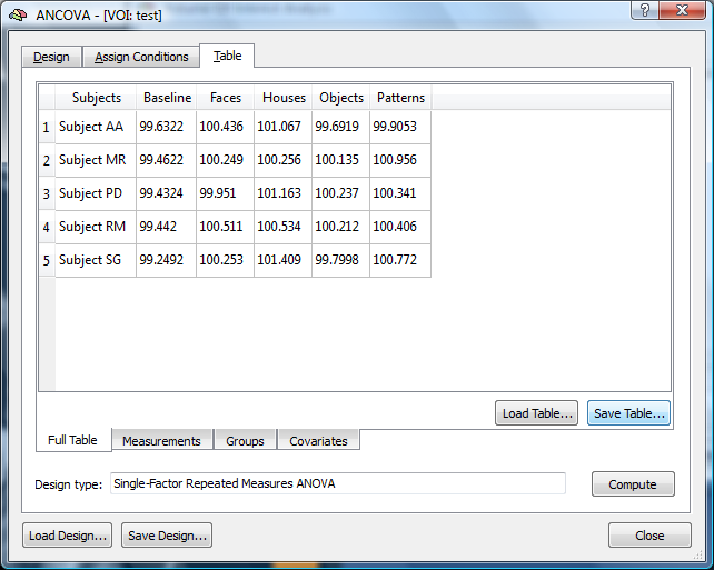
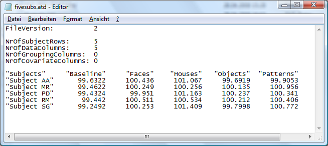
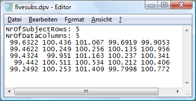
12. 12. With the new table, we could either run different types of analysis or just save the values. On the “Table” tab, we can save the values with the extension DPV. On the Full table tab, we can save the values plus column names as an ATD file.

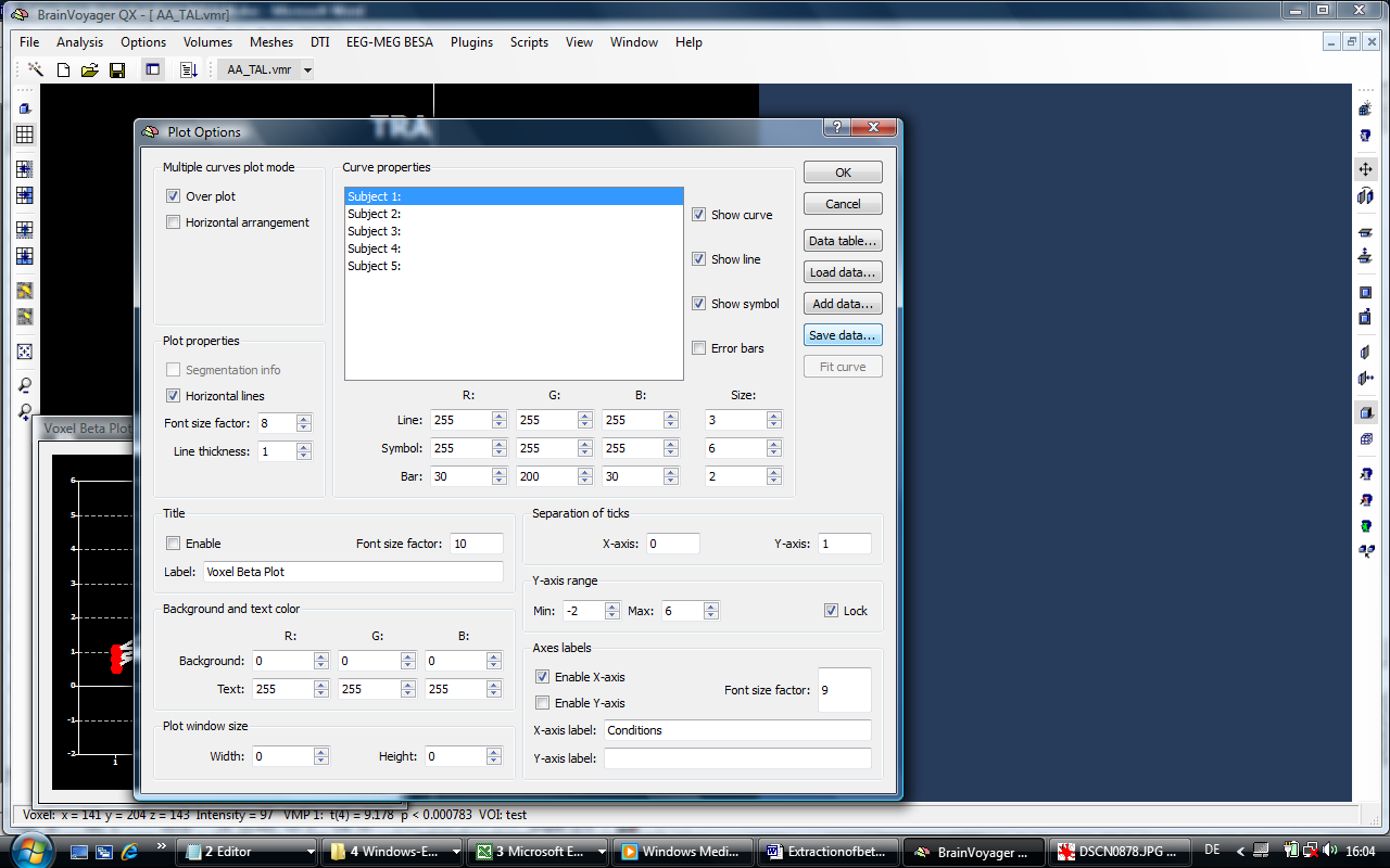
13. 13. As a third way to extract the betas, we use the voxel beta plot option in BrainVoyager. This allows us to get an immediate overview of the beta values of each condition and voxel. We position the mouse over the cluster that was selected before

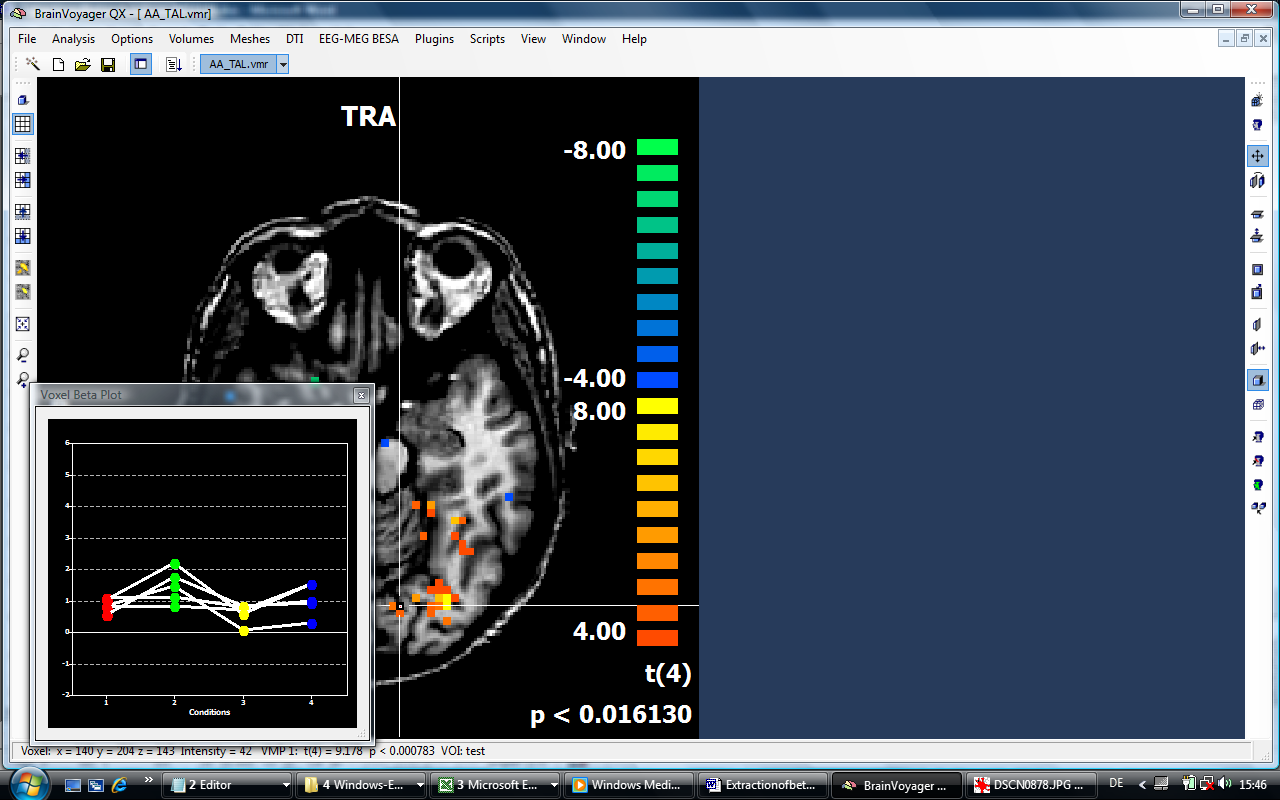
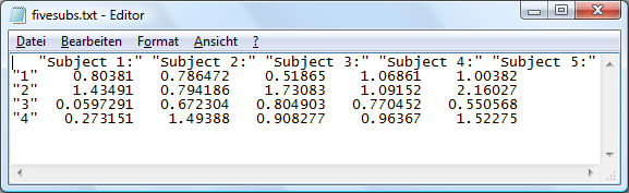
14. 14. To extract the values, we hold down the “Shift” button and move the mouse over the plot. Clicking in the plot allows us to save the data as a simple text file.

15. 15. To compare the value gained by the different methods, we first have to understand the differences between the different formats.
    
    a) Voxel beta plot: in the voxel beta plot, the beta weights are “cleaned” for the mean signal level/confound vaue. The following screenshots shows the results beta extraction

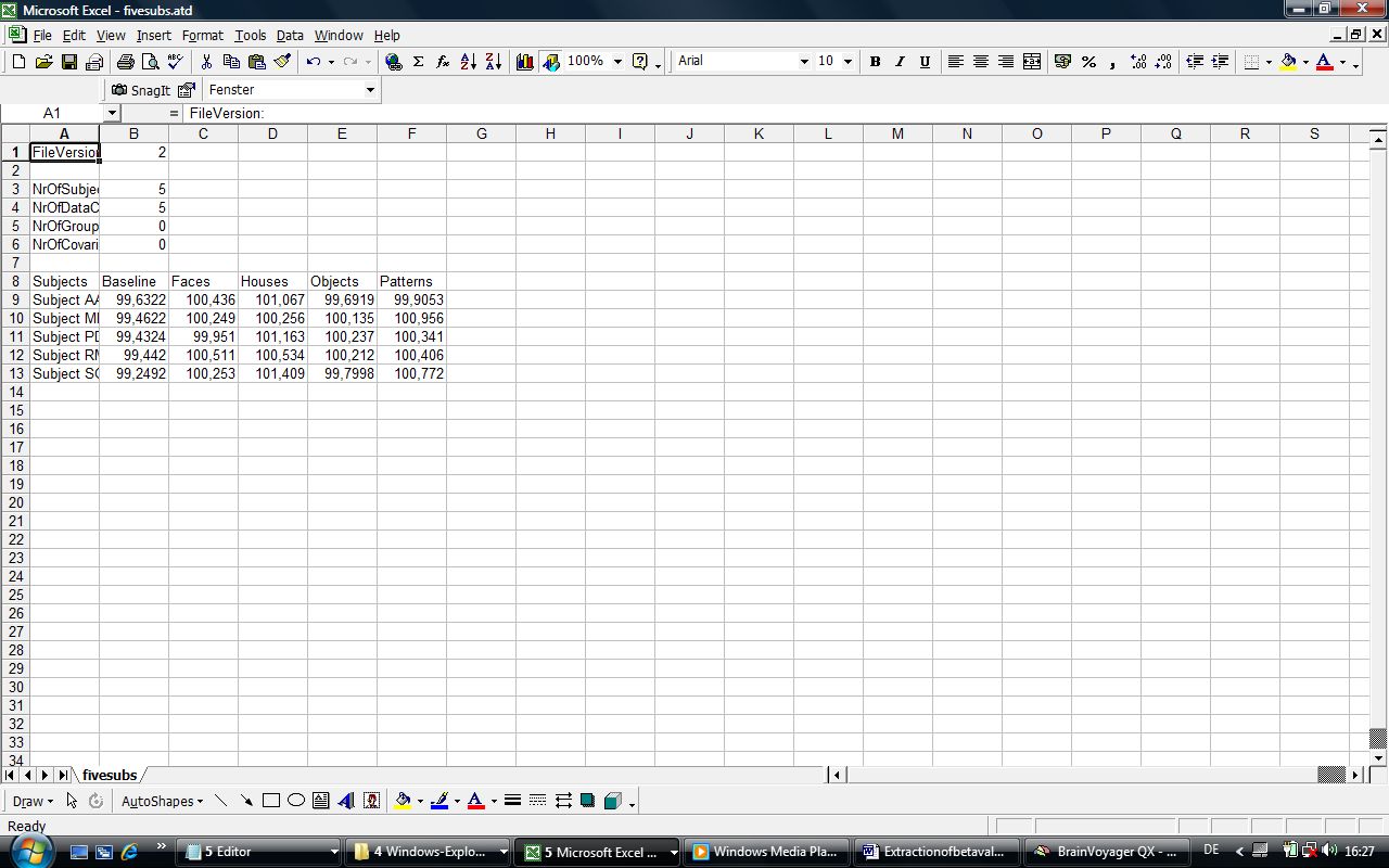
1. b) ATD and DPV files: In the files, the beta values are displayed together with and in relation to the baseline values: To obtain the “cleaned” values, one has to subtract the values in a certain predictor column from the value of the baseline column.

16. 16. Validation of values:

To check if the values in the different formats are corresponding, we use Excel to import. Here, we import the ATD file created into Excel.

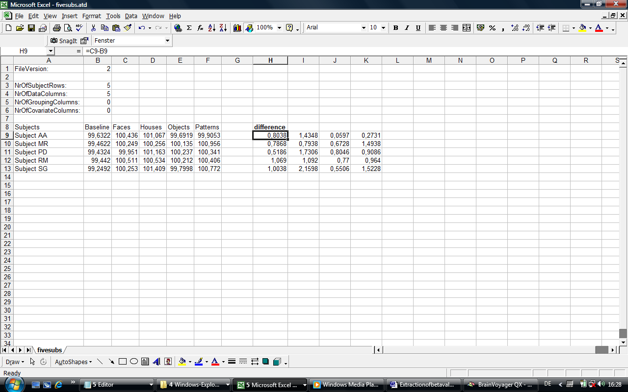
In the next step, we have added a couple of new columns that code the difference between the predictor and the baseline columns.

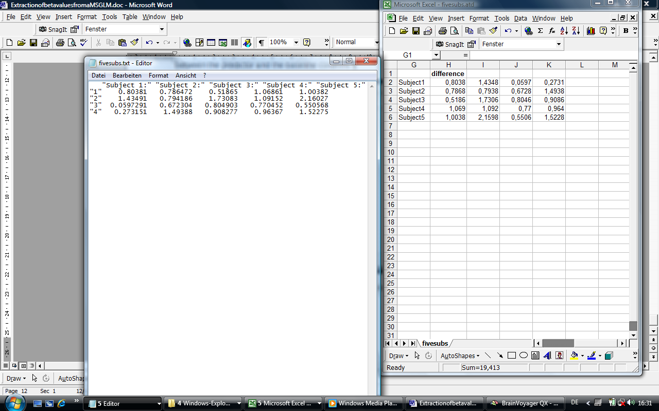
We compare the values to the values in the voxel beta plot: The only difficulty is that internally, we have to transpose the columns and rows of the Excel sheet because the subjects and conditions are coded the opposite in the result file of the voxel beta plot (Rows correspond to conditions in the voxel beta plot file and to subjects in the ATD file). Apart from that, it can be seen that the values are corresponding.

We also compare the Excel file to the previously created ROI HTML file. Again, the same principle of comparison applies and again, we receive a satisfying result.

• Prev
• Next