1.8 Fiber Tracking

1.8.1 Interactive Fiber Tracking

Interactive fiber tracking is meant for exploring the tracts. In real-time, you are able to “draw” fibers on a slice. BrainVoyager puts seedpoints on the location where you click. Using all that you know now about DTI analysis in BV, this is done as follows:

1. Open a VMR
2. Open a DDT file
3. (optional) calculate FA/MD maps
4. Go to DTI --> Fiber Tracking and Rendering
5. Display a slice by using the buttons from table ??
6. use Ctrl+Left mouse click to paint fibers on the slice

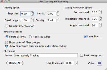
Since the method is interactive, it’s very useful to test the various fiber tracking parameters. The table below shows the parameters and their meanings. Depending on your application, you are encouraged to play around with the parameters.

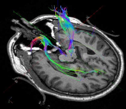
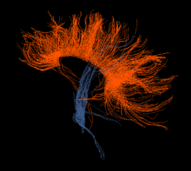
In the end, you’ll end up with an image like this:

1.8.2 Fiber tracking from seed regions (VOI/ROI)

Fiber tracking can also be started from anatomically or functionally (fMRI) defined regions, usually termed regions of interest (ROI) or volumes of interest (VOI). We will use VOI here, since the VOIs can be defined in 3D.

Anatomically defined VOIs Anatomical VOIs are defined by drawing them on a VMR with or without an overlayed FA/MD map.

Open a VMR and the DDT file as explained before. Overlay a FA/MD colormap of your choice. For this demonstration, a FA map is overlayed, color coded according to the maximum values. Next, go to the VMR and open the 3-D Volume Tools dialog. Go to the Segmentation tab.

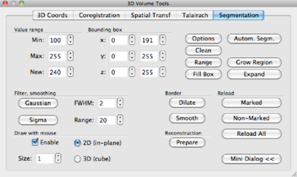
In the Draw with mouse section on the lower left of the tab, check the Enable box. We have now enabled a drawing pen, and the properties of this pen can be changed 1) by size and 2) 2D or 3D: in 2D, the pen draws a square ie 2 × 2 voxels, in 3D a cube with dimensions set by Size, ie 2 × 2 × 2 or 3 × 3 × 3 voxels.

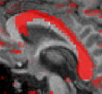
In the VMR window, you can now draw with Ctrl+Left mouse click. But beware! Since the VOIs you are drawing are seed regions for DTI fiber tracking, the borders of your VOIs need to be limited by the DTI data, and not by the VMR data. The DTI data (acquired with a DW-EPI sequence) is distorted relative to the T1 anatomical data. This is illustrated below. The red color shows high FA in left-right direction overlayed on T1 anatomy.

A VOI can be drawn now on the corpus callosum using Ctrl+left mouse click. With Shift+left mouse click, voxels may be removed from the VOI. When drawing is finished, click the Options button on the Segmentation tab. A new window pops op, click the Define VOI button. Then you’ll be asked to enter a name for the VOI. Type a name, and click Ok. The VOI analysis window is now shown, displaying all currently defined VOIs.

When you would like to draw a second VOI afterwards, select all current VOIs and click Hide VOIs. Also, click the Reload All button in the segmentation tab. If you don’t do this, the new VOI will be added to the visible VOI. A new color is automatically assigned to the VOI. Examples of VOIs in the corpus callosum and cortico-spinal tract are given in the figure below. The VOIs can be saved by clicking the Save button.

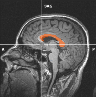
(a) VOI at the corpus callosum in orange.

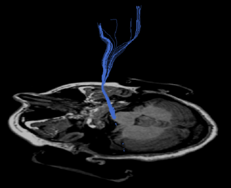
(b) VOI at the brainstem for the corticospinal tract in blue.

Figure 1.7: VOIs

Next, set the parameters for fiber tracking in the DTI --> Fiber Tracking and Rendering window. Fibers from these VOIs can be tracked via DTI --> Track fibers from VOIs.

The appearence of the fibers can be changed, to result in the following images:

(a) Fibers as lines, color according to seed VOI.

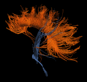
(b) Fibers rendered as tubes

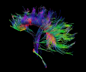
(c) Fibers rendered as tubes and direction color coded.

Figure 1.8: Different visualizations of fibers.

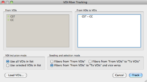
Using multiple VOIs BrainVoyager can also track fibers from and to multiple VOIs. Suppose we have defined 3 VOIs: A, B and C. The following operations are permitted, when ticking the ‘‘From VOIs to VOIs'' radio button in the VOI Fiber Tracking dialog:

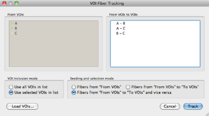
AB
AC
BC

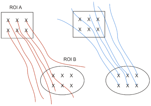
The advantage of using the last option is that in potential more fibers are found. This is illustrated in the figure below. When tracking from A to B, only 3 fibers are found which go through A AND B. When tracking in the reverse direction, from B to A, 5 fibers are found. Combining the two results in 8 fibers.

1.8.3 Spatial Transformations of fibers

ACPC/TAL Transformation Fibers may be transferred into ACPC or TAL space from native space. In this case, the only thing that is transformed, are the fiber bundles. There is no transformation of the original diffusion weighted data, as happens when you would transform the original DWI data into TAL or ACPC.

In order to do this, you need to bring the VMR into ACPC or TAL space. The transformation files that are created by BV during these steps are used now to transform the fiber bundles.

ACPC transformation In the DTI --> Spatial Transformations dialog, click Load .TRF, to load an <subject>_ACPC.TRF. Click the Apply button to perform the transformation and OK to finish.

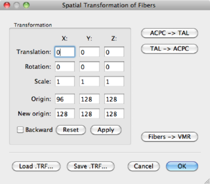
Save the fibers as <subject>_ACPC.fbr.

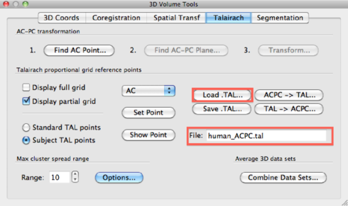
TAL transformation After the ACPC transformation, you can apply a Talairach transformation. To do this, load the <subject>.TAL file in the 3D Volume Tools > Talairach > Load .TAL dialog. The TAL file name will show up.

Then, go to DTI --> Spatial Transformations and click the ACPC -> TAL button and OK to finish.

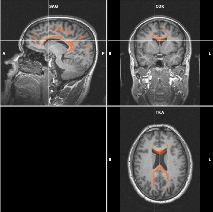
Backprojection of fibers to the VMR It is possible in BV to evaluate the fibers directly on the VMR, in 2-D space so to say. Again, be careful, the fibers may be distorted relative to the anatomy! In the DTI --> Spatial Transformations dialog, click the fibers -> VMR button and BV projects the fibers onto the VMR slices in the same colors as the fibers (that is, ROI colors). In the figure below, the result of such a backprojection for the corpus callosum fibers is shown. This backprojection leads to a new VOI, so it can also be used to get statistics from fibers, as explained in the next section.