Usage of the ClusterThresh Plugin

Prerequisites. Before starting the ClusterThresh plugin, load a VMR file and compute or load a VMP file. Any volume statistical map (e.g., t-, r- or F- map) is internally represented as a VMP. Adjust the single-voxel threshold in a way that you get a "good" map, e.g. with p-values in the range of 0.01 - 0.00001 (uncorrected). The specification of the initial single-voxel p-value is necessary because of the subsequent Monte Carlo simulations.

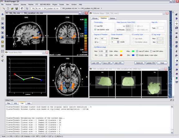
As an example, the snapshot below shows an overlayed VMP (directly from a GLM contrat) which is thresholded at p = 0.005. The "Volume Maps" dialog shows that there is a VMP available and gives you the control of the voxel-level threshold. It is also a good practice to define a mask file which might be useful during the plugin run (see snapshot and below).

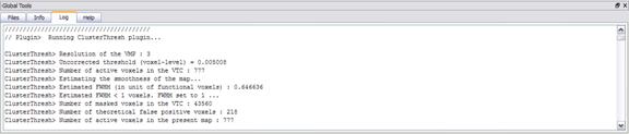
To start the plugin, simply click on "Cluster-level Statistical Threshold Estimator..." in the "Plugins" menu and follow the instructions. Since results as well as problems are reported in the BrainVoyager QX Log tab, you should have a look at the text output written to the Log. The plugin guides you through the four stages of the procedure: image generation, image smoothness modeling and estimation, masking (optional) and Monte Carlo simulation.

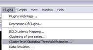
Image generation. The process of 3D image generation is simulated by filling a volume with independent normally distributed random numbers. The volume and the resolution for the image generation corresponds the dimensions and the resolution of the current VMP (native resolution). Please note that the possible interpolation of the overlaid VMP to the current VMR resolution (normally 1 mm), which can be controlled by the user, is only valid for visualization purposes. In order to visualize the native resolution of a VMP simply uncheck the interpolation button in the Overlay VMP dialog. The native resolution of VMPs used for the calculations of the statistical maps is also used for the simulations.

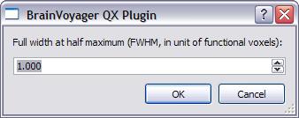
Image smoothness modeling and estimation. The 3D spatial correlation structure of the current VMP inside the 3d box of definition and at the native resolution is estimated and modeled assuming a normal distribution of the underlying population of voxel intensities. The full-width-at-half-maximum (FWHM) of the equivalent Gaussian kernel for this model is estimated using the 3D extension of the formula reported and discussed in Forman et al. (1995). You can either use the estimated smoothness for the simulation (default choice) or force any other value for FWHM.
Note that the FWHM value must be specified in units of functional voxels, i.e. the native resolution of the VMP data. This means that if the native resolution is 3mm (e.g. 3x3x3 Talairach mm voxel size), a value of 1.382 for the FWHM corresponds to an isotropic Gaussian kernel of 4.146 mm. Each random image generated during the simulation is, thus, convolved with the specified Gaussian kernel to simulate the spatial correlation of voxels. Subvoxel FWHM are not allowed, so a minimum value of 1 voxel is assumed even if the estimation produces lower values.

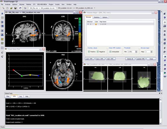
Masking (optional). The VMP dimensions are normally (automatically) specified within a 3D bounding box (e.g. Talairach bounding box). It might be beneficial, however, to further reduce the number of considered voxels, e.g. considering voxels in the brain, voxels within the cortex or voxels with regions-of-interest. For this purpose it is possible to specify at this stage a mask file (*.msk), which will be applied to the filtered random images prior to the thresholding and clustering stage (see below). Note that only masks with the same native resolution of the VMP are accepted. If you want to use a mask file, click "Yes" in the appearing dialog. You will then be asked to locate and point to the mask file. If you do not want to apply a mask, simply click "No".

Monte Carlo simulation. Monte Carlo simulation is performed by iterating the processes of image generation, gaussian filtering, image scaling and thresholding (see below), image masking (optional) and clustering. This simulation step results in a table of cluster size “frequencies”, i.e. it records how many clusters were found with 1, 2, 3... contiguous voxels in the generated “noise-only” volumes.
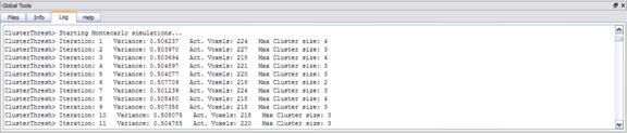
The number of iterations of the simulation must be specified. A minimum of 1000 iterations is advised to achieve an acceptable resolution of the frequency table. The table is interpolated to estimate the cluster-level thresholds event at the anatomical resolution. The number of iteration affects the accuracy of the simulation and the total duration of the computation time. The Log tab informs about the progress.

For each iteration, after gaussian filtering, the image is scaled with respected to the sample mean and sample standard deviation. Then, the image is thresholded such that, approximately the theoretical number of “false” positive voxels are activated in each random map.

Based on the clustering, a tabulation of cluster size frequencies is, finally, reported in the Log tab together with an estimate of the overall significance level achieved for the various combinations of the current voxel-level probability threshold and all the cluster size thresholds within the spanned interval. In addition, the values for the cluster-level probabilities (alpha) are log-transformed and linearly interpolated.

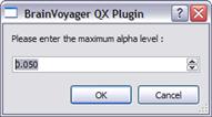
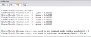
The minimum cluster-size for the user-specified confidence level (alpha) is reported according to the original table (in voxels) and the interpolated table (in mm). This value is also applied to the VMP. A file called “ClusterLevelCorrected.vmp” is automatically saved to the disk in the current folder with the minimum cluster size automatically set on the estimated value.