Part II: White Matter Segmentation
- Details
- Category: Inhomogeneity Correction
- Last Updated: 11 April 2018
- Published: 11 April 2018
- Hits: 9239
This Segmentation guide is a continuation of Part I: VMR Creation and Evaluation
To mark a region of the dataset, we need to open the “Segmentation” tab of the “3D volume tools”.
On the tab, one can find many different options to either automatically of manually select part of the brain. For the moment, we need the options that can be found in the upper part of the dialogue.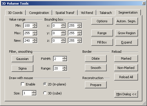
Using mainly two functions, “grow region” and the “expand“, we can mark a selected part of the dataset more or less automatically. To use the region growing procedure effectively, we need to obtain a quick estimate of the material we want to select. To do this, we can just hover the mouse over the interesting types of tissue and inspect the signal intensity value depicted either in the “Info tab” of the global tools (see screenshot) or in the lower part of the BrainVoyager program window. The following screenshots show the intensity in different parts of the dataset.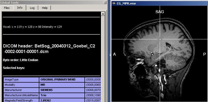
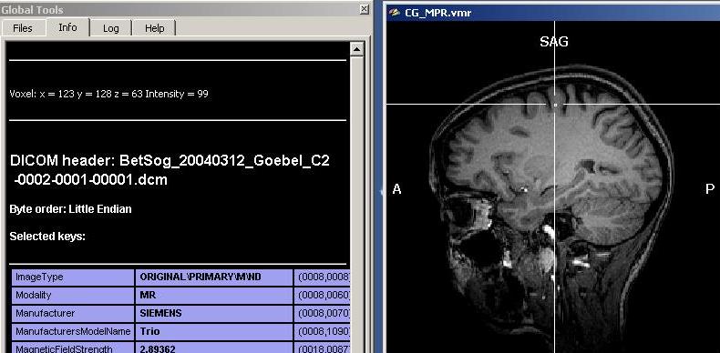
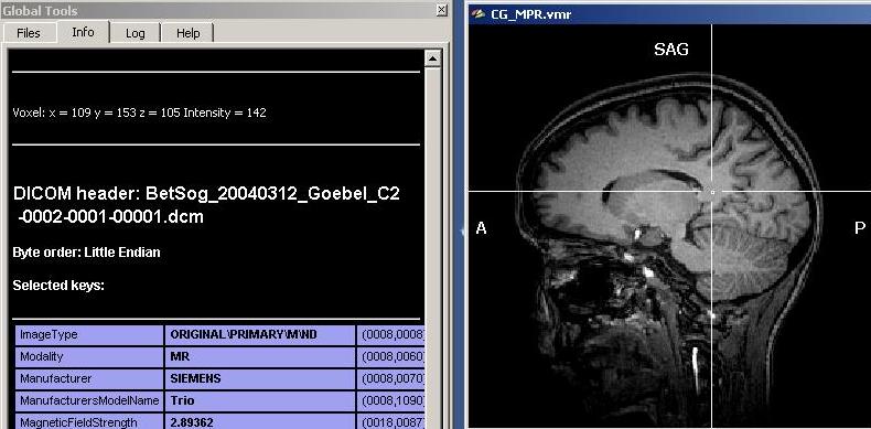
As we can see clearly, there are quite differing intensities at different locations in the white matter (which is already a sign of inhomogeneity). To get a more numerically sound estimation and not just some points, we need to select more voxels of the white matter. To do this, we have to select first a “Min” and “Max” value for the region growing procedure. Because we want to select mainly white, but no grey matter (or other matter types), we select a min value that will surely not touch grey matter voxels. We choose 120 as a “Min” starting value. Too exclude high intensity matter type, we restrict the upper scale of the intensity range, 190 (the precise values in your dataset may be different).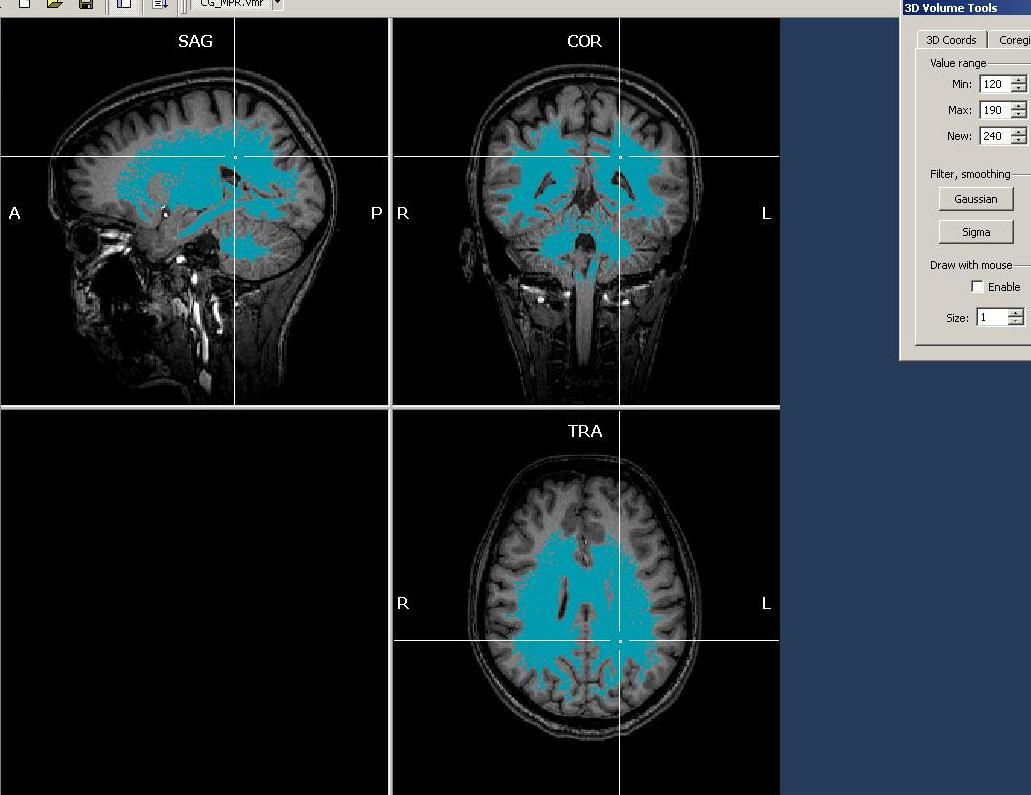
To start the region growing, we have to position the mouse cursor at a voxel whose intensity lies within the specified intensity range. If this “seeding“ voxel has an intensity that is either too low or too high (outside the range selected), nothing will happen. If the region growing procedure selects too many or improper voxels, one can always use the “Reload All” button to return to the previous stage. Unluckily, there is no such thing as an “Undo” button, which means the reload button always gets you back directly to the unmarked dataset.
In this case, the selection between intensity values of 120 and 190 only selects the quite intense voxels in the lower/inferior/posterior part of the dataset.
This is again a sign of inhomogeneity in the data, showing higher intensities in the superior/anterior relative to the other parts of the anatomy. To add more white matter to the selection, we can now use the “Expand” button on the Segmentation tab. Using this button, we only add neighbouring voxels to the already selected voxels, but will not select any voxels not connected to previously marked voxels. To get this method working properly, we have to either decrease the “min” value or increase the “max” value (or both) to cover also voxels that have not yet been selected. First, we decrease the value of the Min value to 110. It is advised to perform rather small steps with this procedure. There are more options to restrict the automatic intensity based region growing, e.g. by specifying a “bounding box” on the segmentation tab.
We press the “Expand” button repeatedly because each neighbour has again a neighbour that may be marked and so forth.
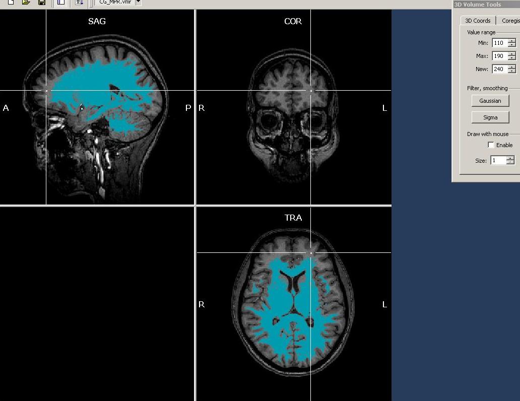
Observing the results, we see that already more, but not all of the white matter has been selected. There are still large parts missing. Hovering with the mouse over the data, we notice that intensity of these (still non-marked) areas is rather between 90 and 110. So we reduce the Min value to 95 and again use the “Expand” button.
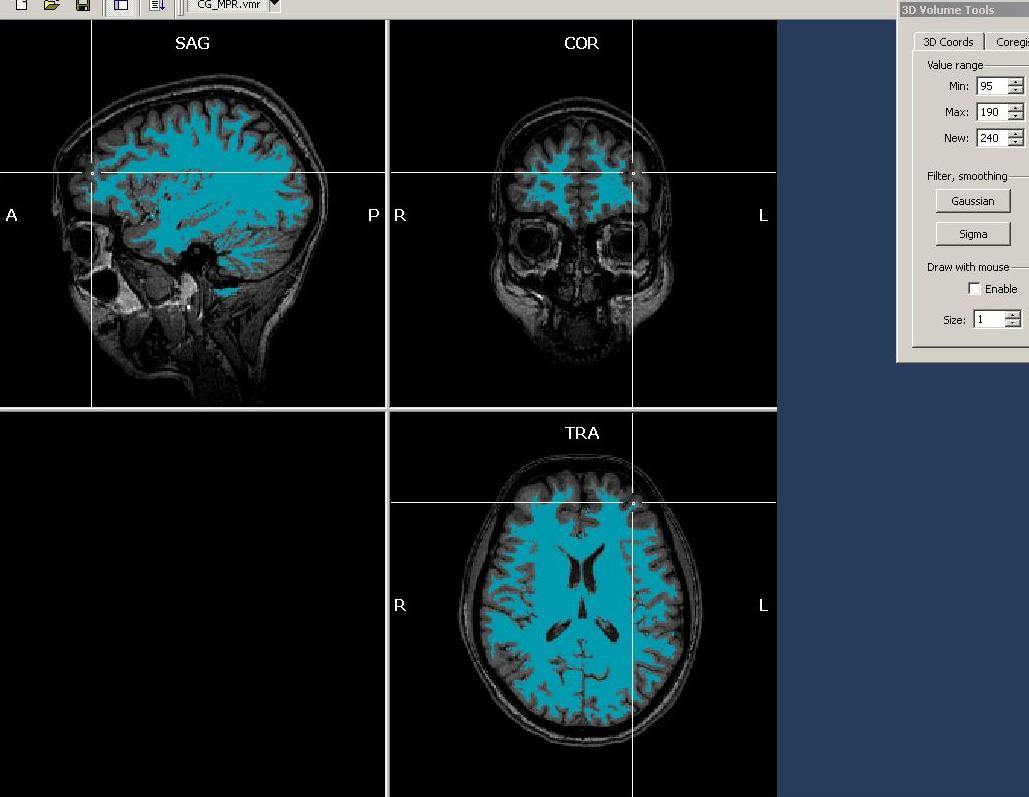
For the moment, we want to inspect a quantitative representation of the voxels just selected. To do this, we open the “Volumes” menu and click the “Intensity histogram” entry.
We obtain a histogram which represents the counts of the differing intensities in two ways. There is a blue graph showing the real counts per intensity value (shown on the x-axis) as well as a yellow plot showing the smoothed version of exactly the same information.
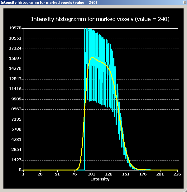
The distribution of the plot confirm the estimation that was already obtained on the basis of the previous inspection, namely, that the intensity distribution of the white matter is too wide and should be corrected. We try to do this is in the next step, the inhomogeneity correction.