Part I: VMR Creation and Evaluatation

When creating a 3D anatomical (VMR) project, BrainVoyager version 1.9.9 will automatically offer to save a corresponding V16 dataset. This specific representation of the anatomy is necessary to perform an important part of the anatomical preprocessing, namely the ”inhomogeneity correction”.

The V16 dataset is a format representing the original greyscale representation of the anatomical dataset. Although visually, this format can not be distinguished from the normal VMR project, it’s an accurate representation of the greyscale information per voxel that is necessary to run the inhomogeneity correction. This depth of information comes with a price: the V16 project is bigger than the usual VMR project. Even users who know for sure that they will never delve into the realm of segmentation and surface reconstruction may still consider to create the V16 file and perform the inhomogeneity correction because this procedure may also help for running e.g. the intensity based part of the coregistration procedure.

When there is any transformation necessary for bringing the anatomy (VMR) into BrainVoyager's standard VMR representation (sagittal orientation, iso-voxel representation, radiological convention), this transformation has to be performed with the V16 project too if one wants to perform the final inhomogeneity correction on the basis of the final VMR result.

BrainVoyager 1.9.9 and later – in comparison to previous BrainVoyager versions - offer to automatically perform the same operations with the V16 file that have to be performed with the VMR dataset. The V16 project can be utilized in the “16 Bit 3D tools” dialog that can be found in BrainVoyager's Options / Volumes menu.

Let’s look at an example of data processing. In this case, we use the same dataset used for the Getting Started Guide (Siemens Trio scanner, MPRage sequence, 192 sagittal slices).

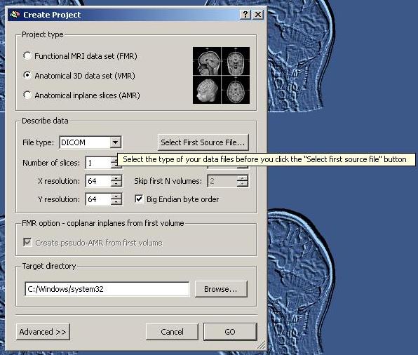
In the “Create Projects” dialog, we select the File Type “Dicom”.

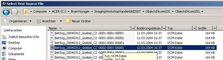
We select the first source file (the DICOM files have been renamed before in BrainVoyager): The anatomical scan was performed in series 2.


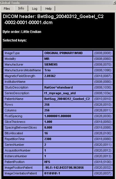
The “Info” tab of the Global tools shows the details gained from the header of the file.


In this case, only the the number of slices (192) has to be filled in manually.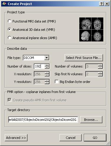

The first view of the VMR project allows us to adjust contrast and brightness of the dataset as well as to save a corresponding V16 file. In this case, we increase the brightness and contrast a little bit. As a rule of thumb, one should try to a) reach a optimal visual representation of the anatomy (no grey background stripe, good grey – white matter separation) and b) obtain a grey matter intensity of around 100. In contrast to that, the white matter should have an intensity between 120 and 150. The contrast / brightness dialog can be reopened at any later point in time via the Options menu. It will automatically save the current settings.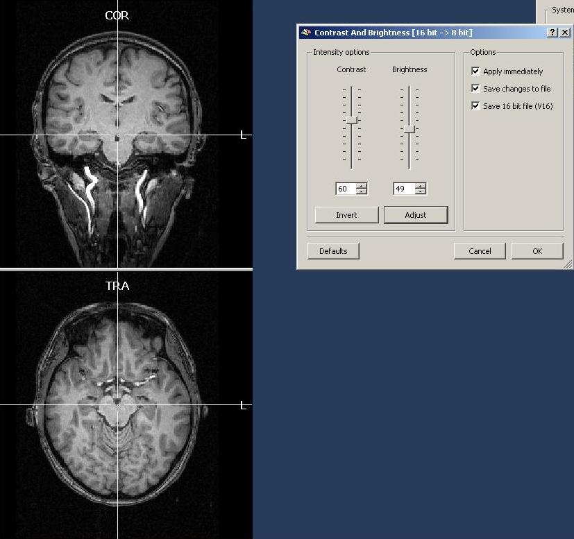
After clicking OK, it is advised to save the VMR project. At the same time, we will also automatically save the V16 project (with the same name as the VMR).

BrainVoyager detects from the header of the data that is has been scanned in radiological convention (left side of the brain is represented at the right side of the image). When the opposite (neurological conventation) is detected instead, BrainVoyager automatically advises a transformation of the data. Whenever a data format is used whose header information is not allowing to obtain this information (e.g. in case of ”Analyze” data), one should be really careful with respect to treatment/interpretation of the side information. In some cases, users utilize external markers attached to the face of the subjects to obtain an absolute side information.

For your own dataset, other transformations, e.g. an iso-voxel transformation or a transformation to sagittal direction, may be necessary. BrainVoyager will automatically advise a new name for the transformed dataset, so the user can always go back an check how the data has been changed. One can always check the spatial properties (and the details of transformation) of the current VMR dataset by opening the “VMR properties” dialog in the “File” menu.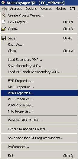


From observing the data, it becomes clear that the brightness of the same type of tissue is not the same in different parts of the brain or in other words the data is still inhomogeneous. 

Options to observe the homogeneity of the data.

a) contrast and brightness settings. First of all, one can open the “Contrast and Brightness“ dialog in the “Options” menu and play around with the settings to check how the intensity of the different matter types is distributed.

To see if some areas of the white matter are brighter than others, one easy approach is to reduce the brightness quite extremely and to check which areas of the dataset stay longer visible than others. In case of a perfectly homogeneous dataset, e.g. every part of the white matter would still be visible up to a certain level of brightness and then become invisible below that level. In case of inhomogeneous data, some parts of the white matter will become “invisible” earlier than others. This can be clearly seen in the screenshot above. The pattern of inhomogeneity depends on the specific dataset and can be quite different.
To not save the current change to the brightness (it is just used for inspection), one just has to click “Cancel” in the “Contrast/Brightness” dialog. 

b) A second option to check inhomogeneity in the data is to mark a part of the brain tissue, e.g. parts of white matter and to inspect the the numerical values of the demarcated region. How this can be done is explained in Part II: White Matter Segmentation