Analysis: Separate Subject & Random Effects

If one wants to compare effects between subjects to be able to generalize the results to the so called population level, a Random Effects approach is necessary. In the Random Effects approach, the different subjects are treated as random samples from the possible selection of subjects (whereas the subject factor is fixed in the Fixed Effects analysis), which leads to a critically different Design Matrix. Nowadays, the Random Effects approach has become a standard in fMRI analysis. Note, that for generalization to the population level, many subjects should be included, i.e. in non-fMRI related studies 50 or more per experimental group! With a few subjects, it is simply impossible to estimate general population effects. The recommended minimum for random effects analyses in fMRI studies are 10 subjects per experimental group.

In BrainVoyagerQX , there are two possibilities to do a Random Effects Analysis:

New RFX approach

This analysis immediately calculates beta weights per subject and predictor (so you don’t have to change the options at the overlay GLM stage). The new approach is technically improved and allows the calculation of very large studies in a reasonable time (which sometimes presented a problem in following the second way described below in prior versions).

In order to successfully separate the subject predictors, the program has to know which VTC files belong to which subject. To ensure this, the names of the included VTC files must follow a simple rule: All VTC file names belonging to the same subject must begin with the same piece of text coding the subject. This subject coding section of a VTC file name is defined as all letters from the beginning of the file name up to the first encountered underscore ("_"). An example of a correct naming scheme is shown here:

• BS_EXPX_RUN1.vtc
• BS_EXPX_RUN2.vtc
• ML_EXPX_RUN1.vtc
• ML_EXPX_RUN2.vtc
• ...

In this case, the first two file names would be assigned to subject "BS" and the third and fourth file name would be assigned to subject "ML". Instead of the initials you can also use numbers. The file name scheme used in the example above is

• "<SUBJECT-NAME >_<EXPERIMENT-NAME>_<RUN-Number>.vtc"

while only the first section up to the underscore is crucial for the subject sorting.

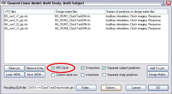
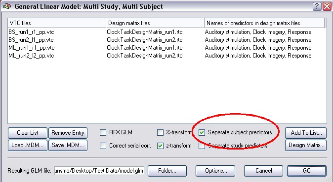
To do the new RFX-analysis you have to use the RFX GLM checkbox in the Multi Study GLM dialog. This automatically checks the %-transform (timecourse normalization) and the Separate subjects predictors checkmarks:


We can now inspect the multi study design matrix reflecting the separate subject predictor settings. Click the Design Matrix button. After clicking the Zoom out button several times, the design matrix should look as shown in the following figure: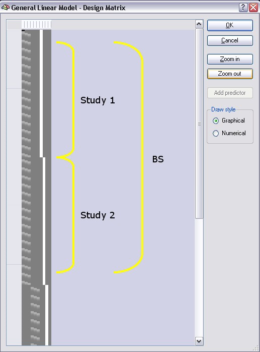 

As you can see, there are now two sets of the three main predictors. Each predictor set defines a time course (non-zero values) for two studies each belonging to one subject but contains zero values (dark grey color) for all other studies. Each subject, thus, has its own set of separated predictors. As before, the design matrix segments for the first two studies have been labeled with yellow brackets ("Study 1" and "Study 2"), the time points of the third study are only partially visible and the fourth study is not visible in the figure. Study 1 and two belong to subject BS, the latter two to subject ML.

The separation of predictors for each subject means that the signal changes at a voxel time course are estimated by 6 (2*3) values (beta weights of the main predictors) across the concatenated data points plus the respective constant terms. Since the predictors for a particular study contain, however, only zero values for the other studies, only four values (beta weights of the three main predictors plus constant term) actually estimate the time course of the studies belonging to a single subject. Although the runs belonging to the same subject are explained by one set of predictors, the signal level confounds are still defined separately for each study (see design matrix). To run the RFX-GLM click the GO button. If you then invoke the Overlay General Linear Model dialog, it will look as follows: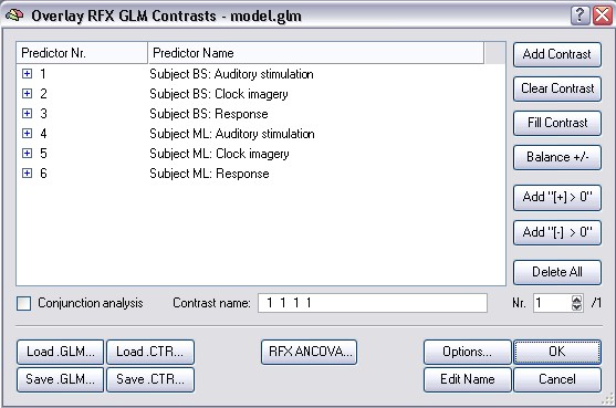



The signal level confound predictors are hidden. The six rows represent the three main predictors for each subject of the multi study design matrix. The three main predictors are appropriately labeled to reflect the subject to which they belong. If you now specify contrasts, the same predictors will automatically be included for all subjects. The resulting contrast map now shows a comparison of the individual betas of all subjects. This way, the variability between the different subjects can be calculated and thus conclusions be drawn also for the general population.
You will notice the degrees of freedom in the right lower corner to be number of subjects-1, in our case one.

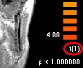
Thus you can easily understand, why a RFX-analysis with less than 10 subjects does not make sense for a real study, here we used it for simplicity reasons only.          

Classical separate subject predictors approach

This way is very instructive, so we explain it here, though for most applications we recommend the new RFX. This classical way is very similar to new RFX, only it uses a two step procedure. It pools the predictors of all studies (runs) belonging to a subject like before. Check the Separate subject predictors option in the General Linear Model: Multi Study, Multi Subject dialog, then calculate the GLM.


In the second step of this approach (the so called summary statistic), a contrast is specified and the Random Effects Analysis is checked in the Options of the Overlay GLM approach.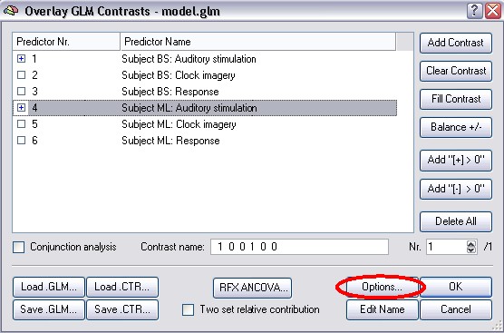 





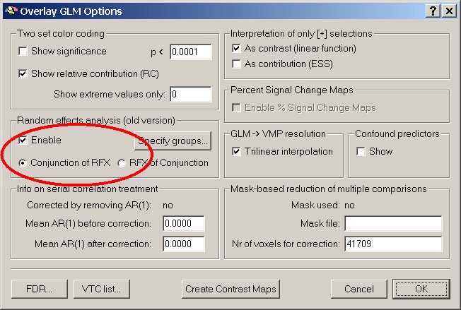
This defines a t-Test for a specific contrast only, so no random effects GLM that includes all predictors, like the new RFX-analysis. For this it uses the beta weights calculated during the first step.