How to analyze multiple VMPs using the “Combine VMP” option

BV version used: BV QX 1.9.10
Dataset used: simulated group data created with the “group data simulator”

Recently, the option to evaluate volume maps (e.g. to check the variability of effects between subjects of a sample) as well as to run basic statistics on the level of volume maps (VMPs) has been facilitated in BrainVoyager. This document describes how to use the so called “Combine VMP” option in BV QX version 1.9.10.

Preparatory steps

First of all, one has to run a statistical analysis to prepare for the following, volume map based analysis. In this case, the “group data simulator” plugin of BrainVoyager was used to create simulated functional timecourses and design matrices to run a Multi-Study GLM. To use this tool, one has to provide a protocol and may create as many timecourses and design matrices as necessary / wished. The group data simulator plugin is described in the corresponding folder of the “BVQXExtensions” folder.

We load the prepared Multi-Study GLM (here, we simulated VTC and RTCs for 20 subjects in total).

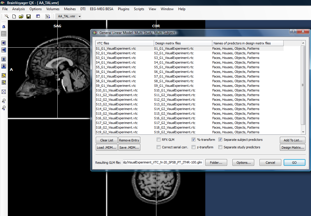
To be able to easily separate the maps of the different subjects in the GLM result, we choose the “Separate Subject Predictors” option of the Multi-Study GLM dialog.

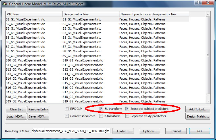
One nice feature of the current BV QX version is that the name of the GLM file created is automatically adapted to the  
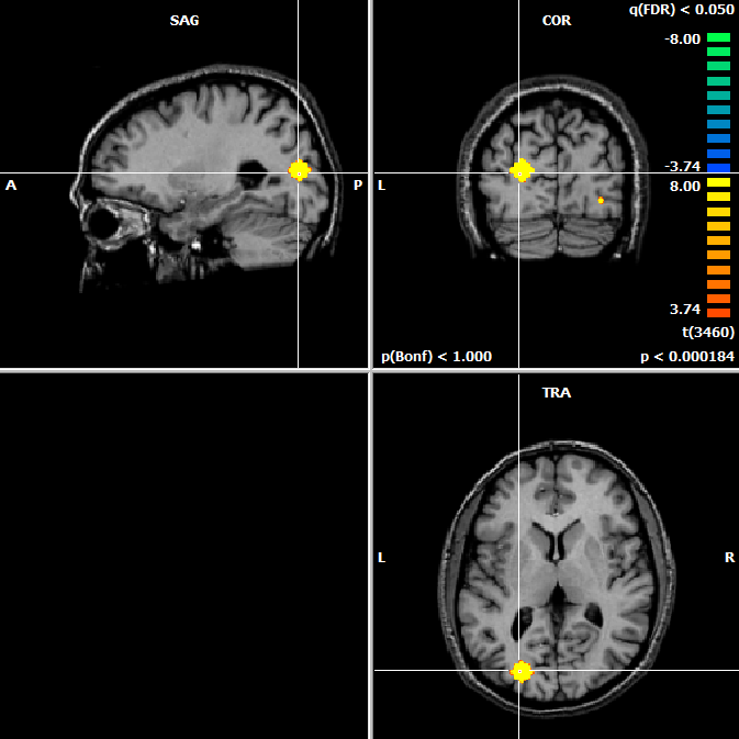
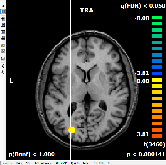
Because the plugin creates the VTC data in a restricted area (to save time as well as harddisk space), only two small localized clusters appears as significant in the statistical map.

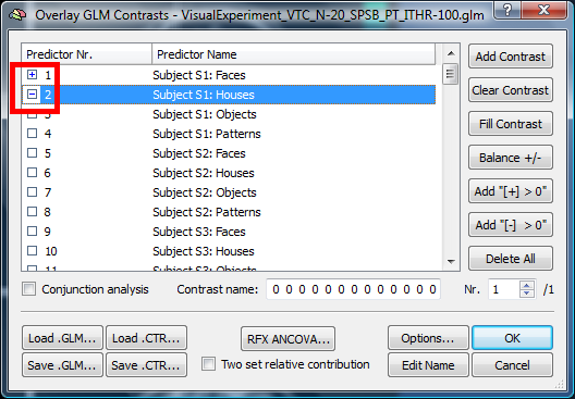
Now, we open the “Overlay GLM” dialog and create separate maps for the different subjects. To do this, we have to check the different subject contrast coefficients.
We start with the first subject:

We check the resulting statistical map:

To create now automatically the same contrast map for all the subjects we open the Options of “Overlay GLM” dialog.

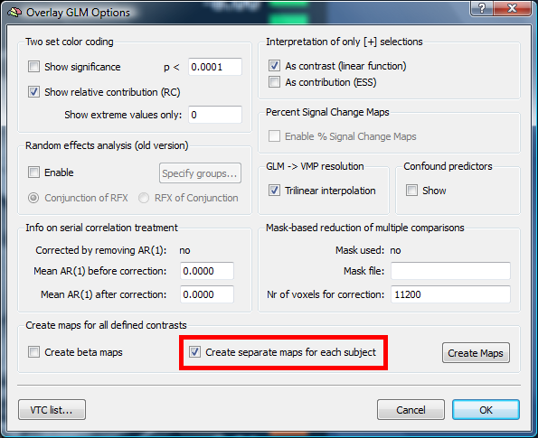
We choose the option “Create separate maps for each subject” automatically generate a map for the contrast chosen in every subject. Now, we just have to click the “Create Maps” button.

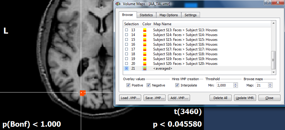
To check the maps, we open the “Overlay Volume Maps” dialog.

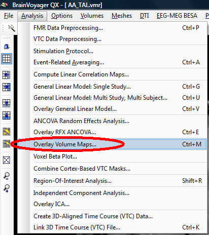
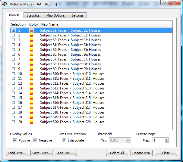
We see that for very single (simulated) subject, the same map (faces>houses) has been created. It is advised to save the volume map at this point (so it can be easily reloaded at a later point). It is a good idea to use a meaningful name, esp. when many different meaningful maps are possible in an analysis.

Now, we can browse the maps one by one or overlay multiple maps by changing the default setting on the “Settings” tab.

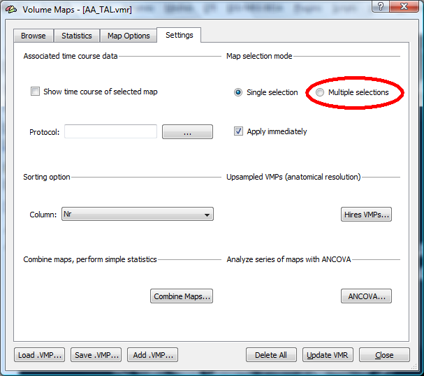
Choosing multiple selections will allow us to overlay multiple maps at a time, e.g. to compare the activation pattern of the subjects.

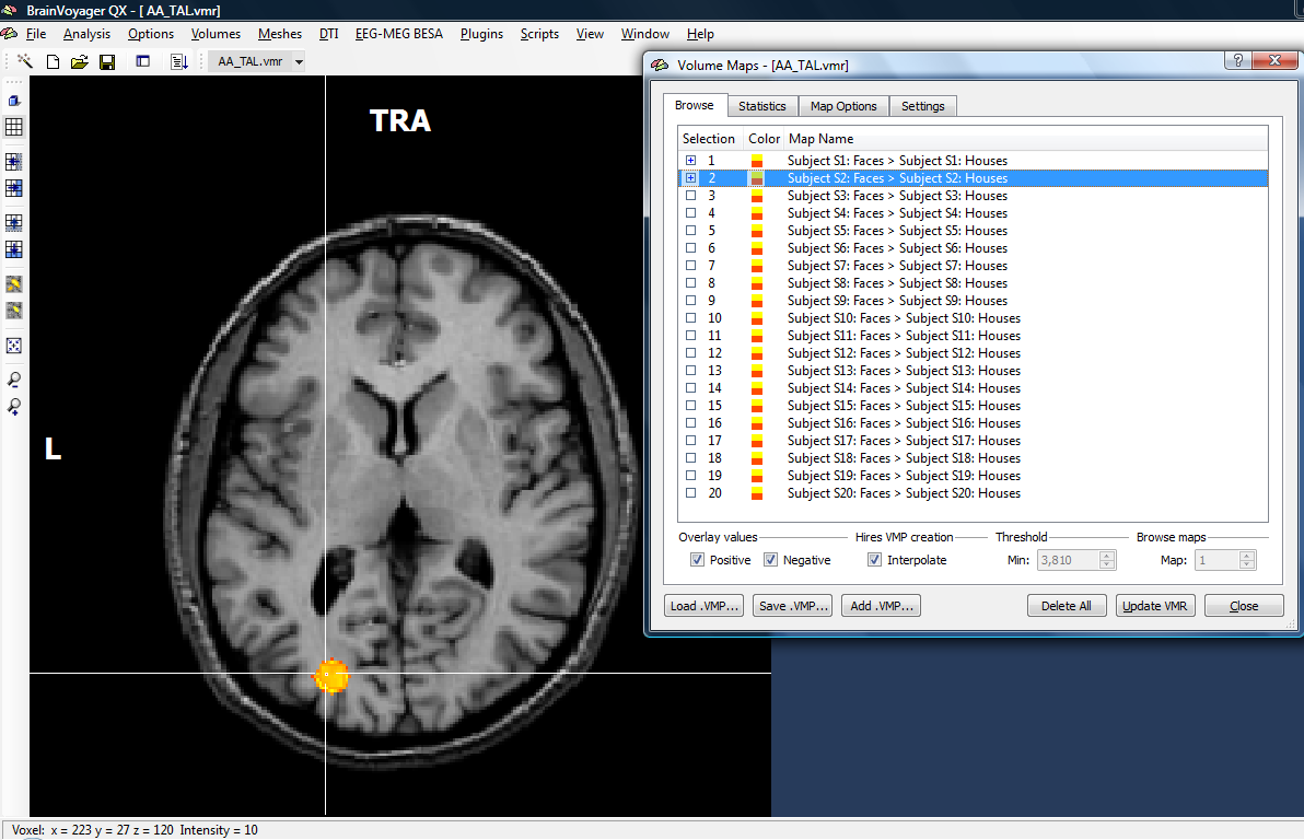
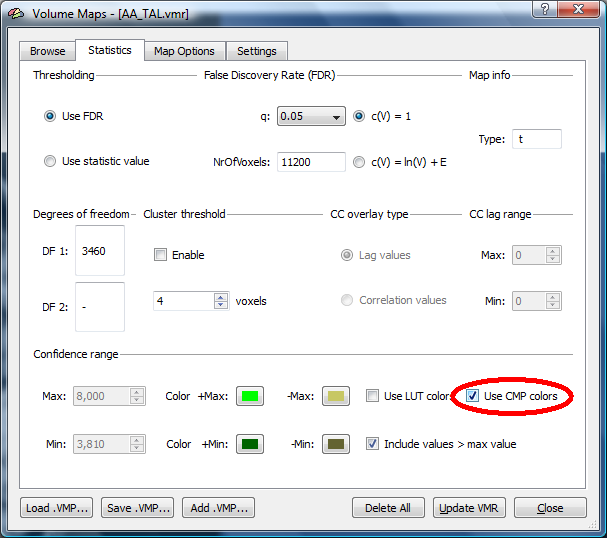
Because it is not possible to disentangle the activation of the two subjects if they are coded exactly in the same way, we can change the coloring of the maps in the “Statistics” tab. By choosing CMP colors, we can freely choose differing colors for the map selected (by clicking on the color plates for min and max values).

In this case we see that the (simulated data) overlaps nearly perfectly.
In a given case, it may also be helpful to turn off the representation of negative values to make life a little easier.

It clear to see that all the maps are based on a different t-threshold, which is according to a respective FDR value of 5% per map. At this stage, one can of course set one and the same minimum t-value for each map.

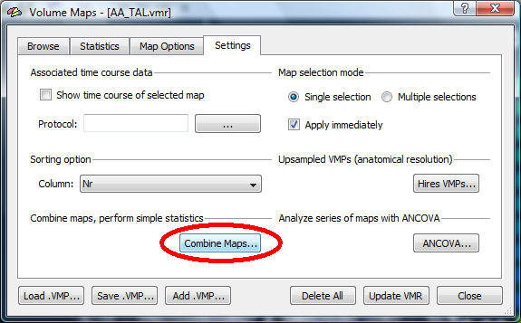
Now, we are able to use the functions of the “Combine VMP” dialog. The button can be found on the “Settings” tab of the “Volume Maps” dialog.

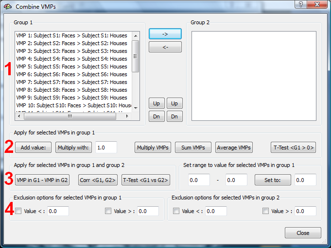
When opening the dialog, one can easily see that generally, it falls into four parts:
1. two list fields that allow to separate the different maps into different groups (G1 and G2). 
2. a second part that can be used to analyze the maps without splitting them into groups
3. a third part that enables specific statistics on the basis of the maps separated into groups.
4. an “exclusion” option that will help to shape specific maps according to their values and a value range selected by the user.

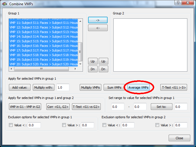
First, we try the statistics that are available for the single group (in the first field). 
We mark all 20 subjects maps and use the “Average VMPs” option.

As the result, a new map will be created in the main dialog (at the end of the map list). We checkmark the map to visualize the result of the average procedure.

The average of the 20 subjects maps nicely shows the difference between the two VOI files that were utilized in the simulation procedure.There was a strong and corresponding effects for the left hemisphere region shown, but a weak and non corresponding for a second VOI located in the right hemisphere. This VOI will not show up in the “average” map. Because of the random noise pattern used, the average will also show muss less noise than one of the single maps.

For the second approach, we switch to the second row to use the group-specific map statistics.

It is important to note three important restrictions for the combine VMP: 
a) whenever the combine VMP dialog is closed, one has to reenter changes that has been made before. There is yet no option to save e.g. group assignments of the VMPs.
b) The maps created with the combine VMPs option can not be deleted from the list of maps in Overlay Maps dialog. One can easily reload the first VMP to recreate the original situation.
c) the maps created with the “Combine VMP” options can not be used to automatically create VOIs via the Options menu. To do this, one could use a specific plugin we can provide. If you want to try this, please send an email to support(AT)brainvoyager(DOT)com

Now, we rearrange the subjects maps into the group fields.
Using the Shift button in combination with the mouse, we mark the maps of subjects 11 to 20 and use the button “->” to shift them into the “Group2” field.

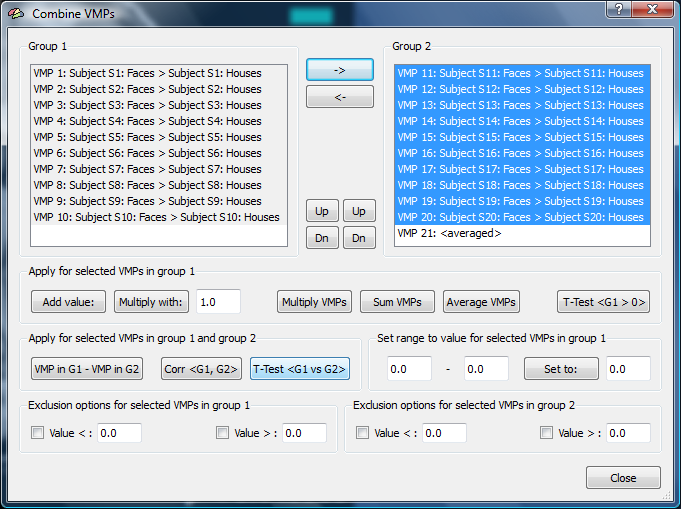
We use first the T-Test <G1 vs G2> button to run a t-test to compare the activation pattern found in the groups. Before doing so, we have to select either all or a subgroup of the subjects (using the mouse). In the moment, it is not possible to delete the previously created map from the VMP file. For the current map statistics, one just has to mark only the maps necessary (S1-S20).
Alternatively one can reload the previous (original) map to clean the former results.
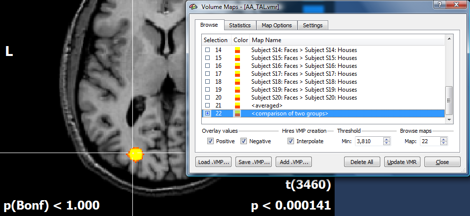
BrainVoyager will again automatically create a new map in to Overlay Maps dialog that contains the result of the specified procedure. We check the map to display its results in the VMR dataset.

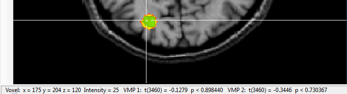
To validate the results externally, we define a single voxel in the significant region an save it as a volume of interest file. In the Options of the ROI Analysis dialog, we can use the VOI Details button to obtain the parameters for all the maps currently displayed.

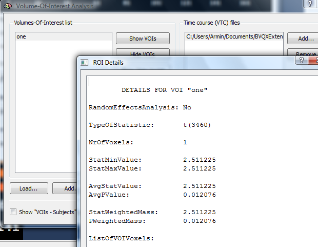
Because the data is quite hard to visualize in the ROI Details window, we import the data into Excel.

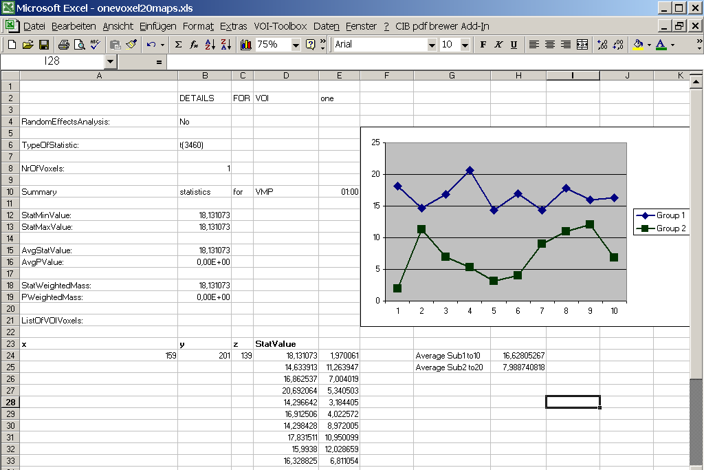
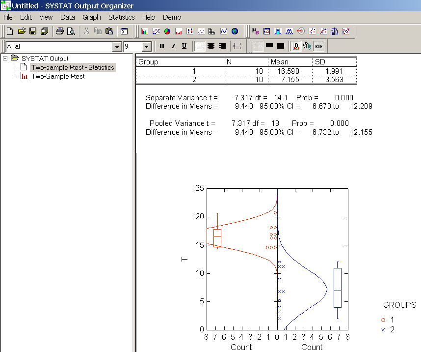
We grouped the obtained t-values into two columns, showing the results of subject 1 to 10 in group1 and 11 to 20 in group 2. Creating a plot shows very nicely the differences between the groups.
To check the statistics, we use the same values to run a two sample t-test in Systat.