Parametric Modulation

Single-Trial Parametric Effect Coding in Single-Study General Linear Model (SS-GLM): Adding “external” factors to the SS-GLM parametric analysis via the extended stimulation protocol and the design matrix builder in BrainVoyager QX 2.1

Introduction

The protocol file (*.prt) contains all relevant information about the experimental design which are needed to start a general linear model (GLM) analysis in BrainVoyager QX. All this information is essential to define the time-course model parameters in GLM analysis.

When preparing a single-study GLM (SS-GLM), the way each condition is transformed to (a) GLM predictor(s) by the design matrix builder (coding) is not unique and should be adapted to what effects are of main interest for statistical testing by the user.

There are four different options for automatic coding of protocol information directly to a GLM design matrix:

1. 1-factor design with dummy coding (default)
2. 1-factor design with effect coding
3. 2-factor design.
4. Deconvolution design.

In a 1-factor design with “dummy coding” (default) all but one conditions (assuming a baseline condition is included in the PRT) are one-to-one coded to a GLM predictor, which will be 1 during the condition intervals and 0 elsewhere (“box-car” function).

A 1-factor design with “effect coding” assumes that each non-baseline condition produces a separate predictor expressing the difference between this condition and the baseline condition. A variant of the effect coding entails with setting up a free coding of multiple conditions in each predictor by manually specifying arbitrary “weights” (via CTRL-right-click) to each condition during a manual definition of the design matrix.

In a 2-factor design the default effect coding is extended from one factor to two factors with the additional option of coding two-factor interactions in extra predictors (i.e. a box-car predictor which is “active” during intervals of activity of one condition and not other and vice versa).

Independently of the condition-to-predictor coding, when building 1- or 2-factor design matrices, the HRF is normally (default) applied (i. e. linear convolution) to the box-car functions.

An alternative to using box-car functions and convolution is the deconvolution design. In this approach, the response to each set of stimuli for each condition can be deconvolved from the data. In fact, in “deconvolution” mode the design builder implements a finite impulse response (FIR) modeling of the event-related responses and each (non-baseline) condition generates a set of stick predictors coding separately the single delays starting from the condition interval onsets.

After GLM estimation, the statistical analysis ends up in translating any linear contrast (e.g. any linear combination of the estimates) into a null hypothesis test of the effects of interest versus 0.

In many circumstances, a parametric question to the data is posed that involve an extra-factor which does not correspond to any of the protocol conditions (e.g. stimulus types). This is the case of pure parametric designs where a “graded” stimulus (e.g. lights of variable intensity) is delivered to the subject or the case when one wants to model the influence or modulation of confound or behavioral extra-factors (e.g. habituation, reaction times, etc …). How should this case be handled in the framework of GLM? How can we optimally integrate some external information from a stimulus grading or an external factor in BrainVoayger QX?

In all these cases, we are still having a standard one factor (stimulus) design but we would like to explicitly test the presence (and the statistical significance) of any possible continuous or categorical effect on the BOLD response amplitude which could be easily interpreted as a parametric “grading” or “modulation” of the response.

We will show below through a simulation how a generic parametric effect by an extra-factor can be tested in BrainVoyager QX. We will consider the most general and interesting case that the parametric effect is modeled at the single-trial level.

Although the parametric effect pertains to the way the conditions and intervals are coded to a design matrix, the most general and portable solution for specifying and storing the values of a parametric extra-factor is not in the SS-GLM but in the stimulation protocol (figure 1).

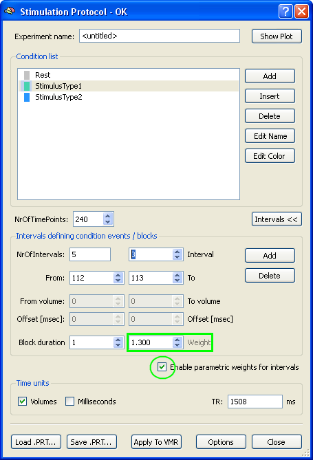
Figure 1

With the release of BrainVoyager QX 2.1, “weights” for the modulation of the predictors and therefore the parametric effect coding can be specified not only in the SS-GLM design matrix builder but inside an extended version of the stimulation protocol. The major advantage of this choice consists in the fact that while in the SS-GLM weights can be assigned to single conditions (i.e. normally groups of trials), in the stimulation protocol different weights can be assigned to all single trials of each separated condition (figure 1).

In standard mode, the new design matrix builder of BrainVoyager QX will now detect the presence of weight definitions inside the protocols and besides generating a standard “dummy” coded predictor for each non-baseline condition (Main), will also generate a “parametrically” coded predictor where each weight will differentially modulate the box car function of the standard predictor (Parametric). As an example, figure 2 shows a simple case with two stimulus types and two modulation types (a linear and non-linear one).

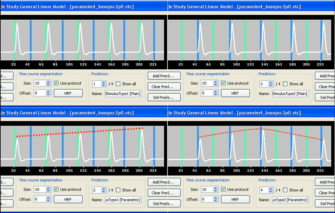
Figure 2

In the example of figure 2 a direct parametric effect coding is shown with the weights specified in the stimulation protocol directly used inside the predictors (before HRF convolution and z-transformation of the predictors).

Please note: z-transformation of all predictors is always assumed here regardless of the specific values of the durations and weights of the single trials inside the box car functions since this ultimately ensures that the resulting predictors have the same variance (balanced design matrix).

Although this type of parametric effect coding is highly intuitive (i. e. directly visualize in separate predictors a non-modulated and a modulated effect), we will here show with the aid of simple stimulation that in most cases of interest this approach is not optimal in the sense of specificity, i.e. for “isolating” form noise regions of activity with statistically significant modulation by an extra-factor.

Simulation

Starting from a real resting-state data set, a new simulated data set was created where the model signals in figure 2 where “injected” in four separated regions.

The usual free parameter of this type of simulations is the “base” percent-signal change of the effect (i.e. the percent-signal change measured in a region with unitary weight). Figure 3 shows the average time-courses of the regions with linearly (left) and non-linearly (right) modulated activity respectively for a base percent-signal change of 0.5% (upper), 1.0% (center) and 2.0% (bottom). The higher the base signal the clearer the parametric effect is visible in the resulting time-courses.

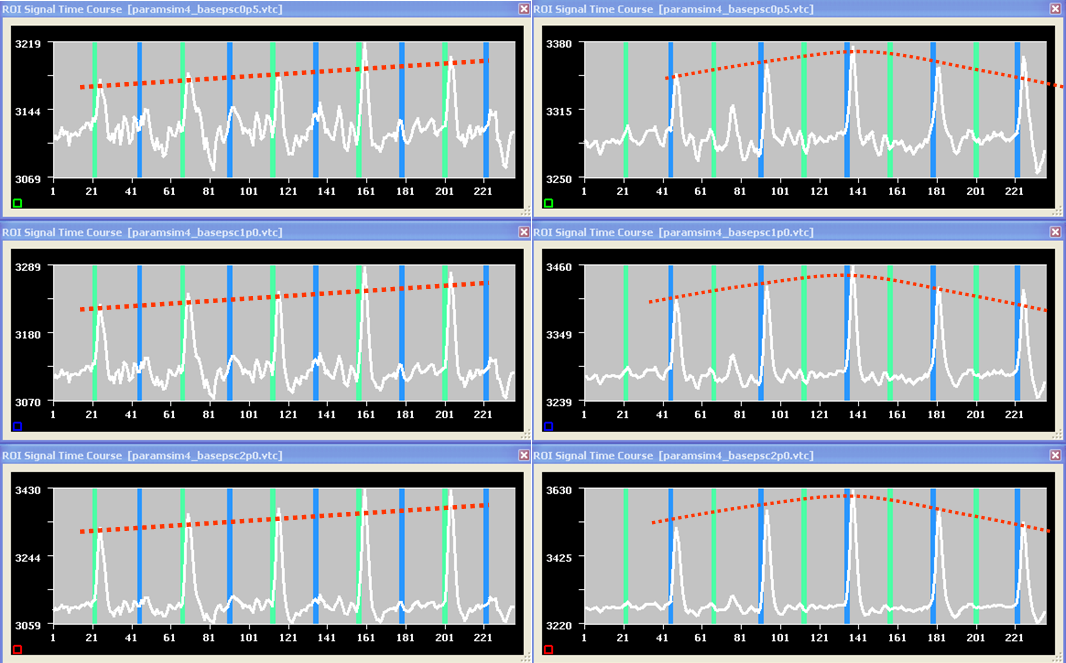
Figure 3

Let us now run a SS-GLM analysis using the design matrix builder but considering not one but two alternative ways of coding the parametric effect. One way is using the same weight for the box-car function as shown above (see figure 2). Another way is subtracting the mean weight before applying the modulation to the box-car function (see figure 4).

Please note: it is possible to control the creation of the parametric predictor by the design matrix builder as shown in figure 2 (“Use weights as defined”) or figure 4 (“Subtract mean of weights”) in the options of the Single-Study GLM Options (figure 5).

The reason why we also use demeaned weights is that this way we can avoid the partial co-linearity between main and parametric predictors in the SS-GLM design matrix. The solution in figure 2 with same weights as defined in the protocol is redundant with regards to this aspect. In fact, since the design matrix is not orthogonal, the parametric predictor will be able to explain a substantial part of the variance regardless of the real parametric effect size. With such co-linear predictors, the isolation of parametrically responding regions becomes more problematic, especially when the parametric effect size is relatively small. Conversely, the solution with de-meaned weights ensures that the correlation between main and parametric predictors is zero (i.e. the two predictors will be orthogonal). In this case, while the detection power (sensitivity) of the method cannot change (because this is related to the signal-to-noise ratio), we will have a powerful method to isolate truly modulated regions via a conjunction analysis of the main predictor and the parametric predictor that now carry complementary information.

We will show here why the solution of subtracting the mean of the weight series before creation of the predictors should be preferred whenever the focus is on isolating the modulated regions (and therefore why this solution is checked as default in BrainVoyager for single-trial parametric effect coding).

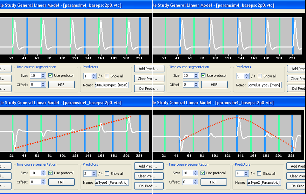
Figure 4

Figure 6 and 7 illustrate two scenarios for the analysis of simulated data sets with base effect size of 0.5% in the region where a modulated response was injected. Specifically, we can notice, that when performing the SS-GLM with the two approaches and selecting the main effect of the parametric predictor (figure 6), the two resulting t-maps are almost identical. We have deliberately chosen here a very low threshold (p=0.05 uncorrected) to explore what will turn out to be an issue of specificity with respect to parametric effect given that our model cannot have an impact on the sensitivity level. The “true” region of modulated activation is shown in the lower left corner of the figures.

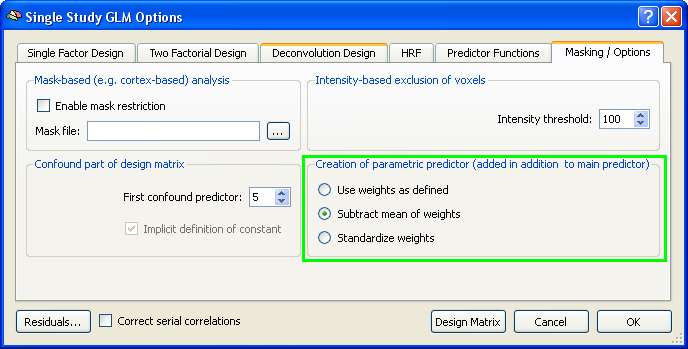
Figure 5

In figure 6, where the main effects of the parametric predictor are tested, besides a true effect detected, we can easily observe many other noisy spots detected at this threshold (false negatives). The false negatives are here due to the fact that the noise fluctuations can easily fit the modulation in the absence of a main response and, unfortunately, this fit can be as good as for the true modulation.

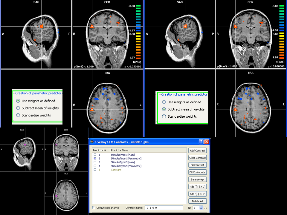
Figure 6

At this point, one concrete chance we have to isolate the true modulation effects from the noise is to require that the region respond not only to the modulation but also the standard main response, in a conjunction analysis. This can be easily obtained by creating two contrasts, one for the main and one for the parametric predictor in the Overlay GLM and specifying a conjunction analysis. In figure 7 we can see the outcome of this conjunction analysis at the same threshold of figure 6.

Keeping the same threshold of figure 6, it is easy to recognize that while all spots are lost for the non-orthogonal case (left), only the true modulated spot region survive the new conjunction test for the orthogonal case (right) where as all false negative modulated spots are lost.

A region of interest analysis (figure 8) in the true spot highlights the underlying reason for this parametric or modulation effect becoming selective in the conjunction analysis with the orthogonal but not with the non-orthogonal design. Namely, the non-orthogonal design (with same weights) explains all variance in the parametrically modulated region with one predictor only (the main is not significant) and makes the isolation of the two contributions not possible or not easy. Conversely, the orthogonal design tells us that both the main and the modulation effects are significant and this does not happen in (most of) noisy spots. That’s why we can exploit the conjunction test for increase the specificity of our design.

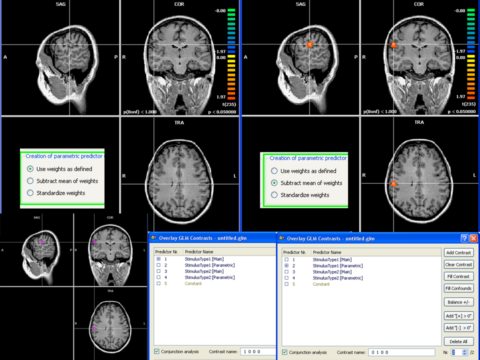
Figure 7

 

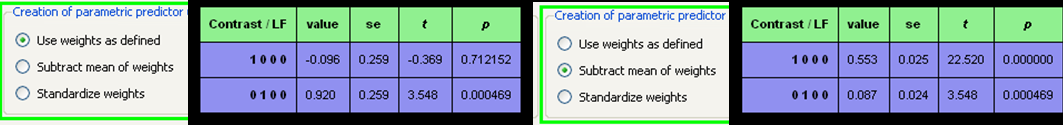
Figure 8

In this example, we manually controlled the scale of the parametric factor. In some applications we might think to use an external measure as extra-factor (e.g. reaction times, physiological responses, rating, etc ...). In all cases where the extra-factor is not controlled by the users but it is rather derived from the data it might be necessary, besides removing the mean, to scale the weights to their standard deviation across trials. And this is what can be accomplished by checking the third option (“standardize weights”).