Brain Innovation

To obtain better insights into how multiple studies contribute to an overall statistical map, it is possible to estimate a separate set of predictors for each study included. After running the GLM, this allows you to compute statistical maps for each individual study as well as for any set of combined studies. In addition, this approach gives you the opportunity to specify study x predictor interaction effects (which isn't common, but can be very useful!). 

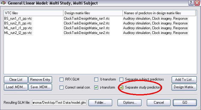
The only change we have to do to switch from the concatenation approach to the separate study predictors approach is to check the Separate study predictors option in the General Linear Model: Multi Study, Multi Subject dialog: 


We can now inspect the multi study design matrix reflecting the separate study predictor settings. Click the Design Matrix button again. After clicking the Zoom out button several times (it might take a while for your dataset, depending on the number of total time points), the design matrix should look as shown in the following figure: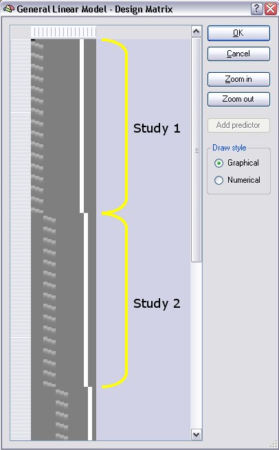 


As you can see, there are now four sets of the three main predictors. Each predictor set defines a time course (non-zero values) only for one study but contains zero values (grey color) for all other studies. Therefore it can be said that each study has its own set of separated predictors. As before, the design matrix segments for the first two studies have been labeled with yellow brackets ("Study 1" and "Study 2"), the time points of the third study are only partially visible and the fourth study is not visible in the figure. 

The separation of predictors for each study means that the signal changes of a voxel time course are estimated by 12 (4*3) values (beta weights of the main predictors) plus the respective constant terms. Since the predictors for a particular study contain, however, only zero values for the other studies, only four values (beta weights of three main predictors plus constant term) actually estimate the time course of a single study. 

This is also reflected in the resulting GLM where you will find 12 main predictors for specifying contrasts. To check this, close the design matrix dialog and run the GLM by clicking the GO button. If you then invoke the Overlay GLM Contrasts and Contribution Maps dialog, it will look as shown below: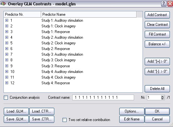 


The twelve filled rows represent the three main predictors for each of the four studies of the multi study design matrix. The three main predictors are appropriately labeled to reflect the study to which they belong. You can now specify contrasts within any single study or across any set of studies providing more flexibility than was available with the concatenation approach. The signal level confound predictors (constant term for each study) are not shown. 

Note: To simplify the specification of the same contrast for each study, hold down the CTRL key while specifying with left and right mouse button clicks the respective contrast for one study. The pressed CTRL key ensures that the defined contrast is copied to all other studies.