There are multiple options to use external variables of interest in the course of a functional data analysis in BrainVoyager. When only one data point per subject is available (compared to the situation of one data point per trial), one can nicely use the correlation tool in BrainVoyagers Ancova dialog.
The procedure is described in this document consisting of 3 sections:
- Preparation
- Correlation Calculation
- External Validation
Preparation
1. First of all, the data has to be analysed in a Multi-Subject “RFX GLM” analysis.
In this case, we don’t use the ordinary sample data, but create simulated data with the “group data simulator” plugin that comes with the standard BV installation.
For running the plugin, a so called GDS file is necessary. This is an editable text file that can be changed to create different kinds of simulated datasets (this way, one can easily create different “effects” to e.g. check if a statistical approach is performing properly).
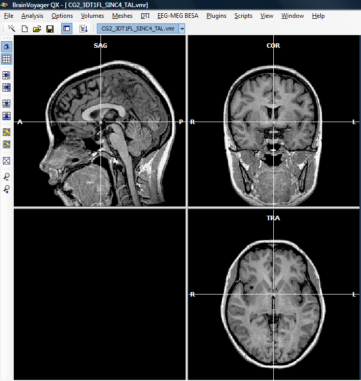
2. To run the plugin, we first need to open a VMR file.
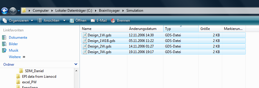
There are a number of GDS files available in the so called “BVQXExtensions” folder after installing BrainVoyager QX (on Windows, this folder is created in the “My Documents” subfolder of the harddisk). In this case, we have copied the files into a new folder called “Simulation”. The new files created by the plugin will be written into the same folder.
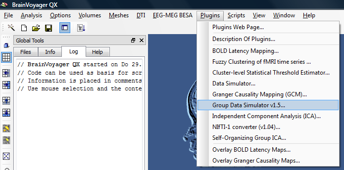
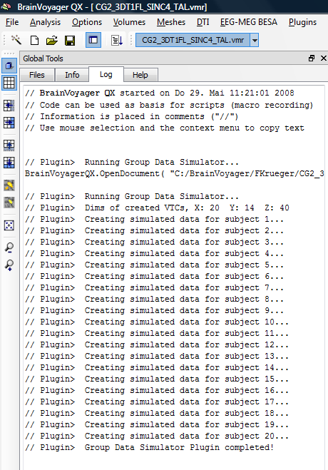
3. We start the group data simulator plugin and localize a GDS file. In this case, we use the file called “Design_1W1B.gds”, which will simulate data for an interaction design containing one within and one between subjects (group) factor.
After running successfully, the plugin has created a specific number of VTC; PRT and RTC files. The process can be inspected in the “Log” tab of the global tools.
4. Before we are able to run a Multi-Study GLM analysis as a preparation of using the Ancova tool, we have to manually create an MDM (Multi-Study Desing Matrix) file.
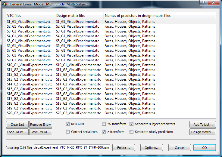
In this case, the subjects are named S[number] while their group assignment is provided in the second part of the name after the underscore (“G1” or “G2”).
5. We run an “RFX GLM“ analysis using z-transformation.
Note that the result is automatically saved in a GLM file whose name codes the details of the analysis (number of subjects, normalisation etc.).
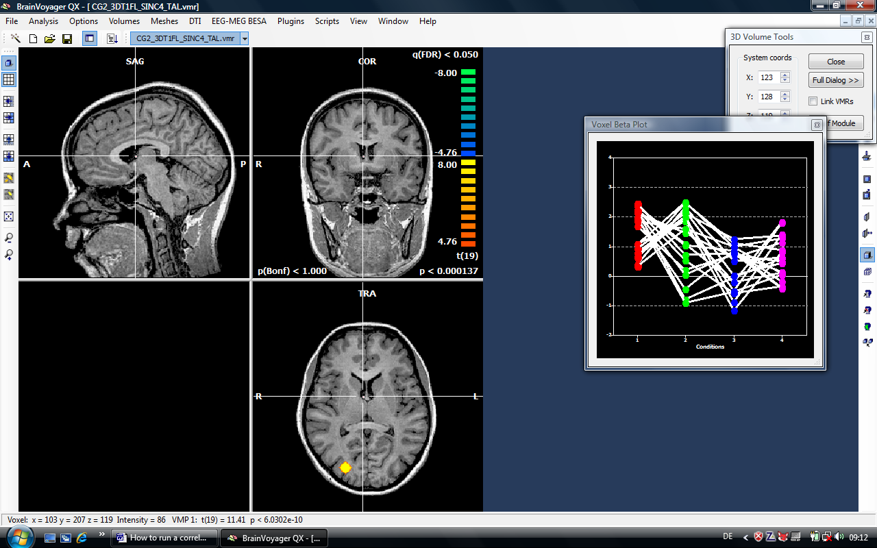
The results looks awkward but is of course based on simulated data (there are only two condensed regions of interest – one in the right hemisphere is visible at the moment). At this point, we can switch to the correlation calculation.
Correlation calculation
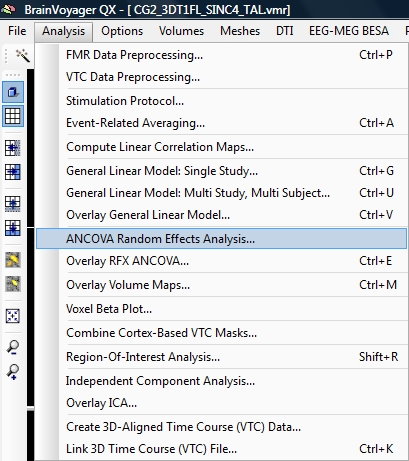
1. We open the Ancova module to be able to run the correlation between the betas and an external covariate.
2. In the first place, the dialog is not properly coding our design (only a within subject factor is represented – based on the predictors of the previous GLM analysis).
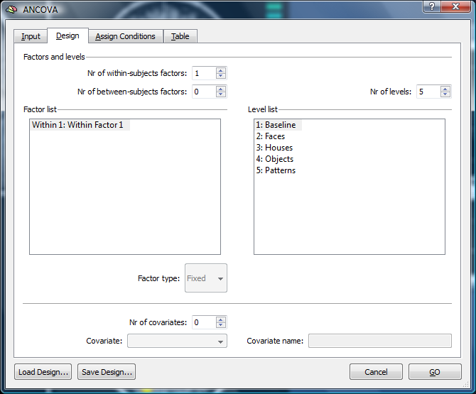
3. For a proper Anova analysis, we would have to add a between subjects factor.
The levels of the within subject factor are based on the number of predictors and the confound. In our case, we have five factor levels (Baseline, Faces, Houses, Objects, Patterns). The number of the within subject factor levels can be adapted to e.g. specify a more simple design. In this case, we don’t add the between subjects factor, but add a covariate to be able to calculate a correlation.
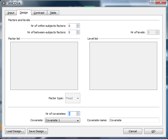
This will add a new tab called “Contrast” to the dialog.
4. We switch to the “Contrast” tab and define a specific contrast of interest. In this case, we specify the comparison of “Faces” minus “Houses”.
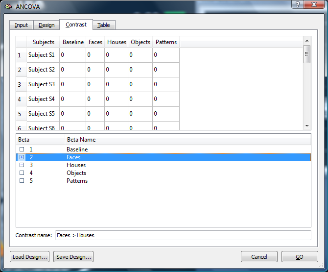
The contrast name (“Faces > Houses”) is automatically displayed in the lower part of the dialog.
5. Now, we have to enter values for the covariate. To do so, we switch to the “Table” tab. The column for the covariate is zero-filled in the moment. The Design Type already provides the description of the analysis (“Correlation between Subject’s Effect (Contrast) and Covariate Values”).
We enter values for the covariate (we use a “pseudo IQ” value). The covariate values can be saved in a format called *.cov for later usage.
To start the analysis, we click the “GO” button.
6. The resulting map contains r-values coding the correlation between the contrast and the covariates values specified:
After running the correlation and creating a full brain r map, we would like to check the underlying calculation.
External validation of the correlation analysis.
1. to avoid interpolation effects, we switch off the interpolation in the “Overlay Volume Maps” dialog.
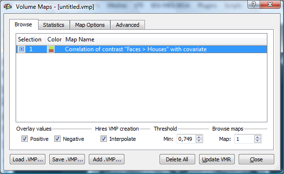
2. The map shows the functional data in it’s native (3mm) resolution.
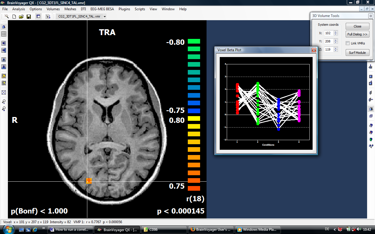
There are multiple options to extract beta value for redoing the analysis externally. We could e.g. extract the values for a single voxel directly from the voxel beta plot or create a volume of interest and extract the values via the options of the VOI analysis tool. In the case, we select the faster approach a. In the task bar of BV, we can inspect the r value at the current voxel (0.7792).
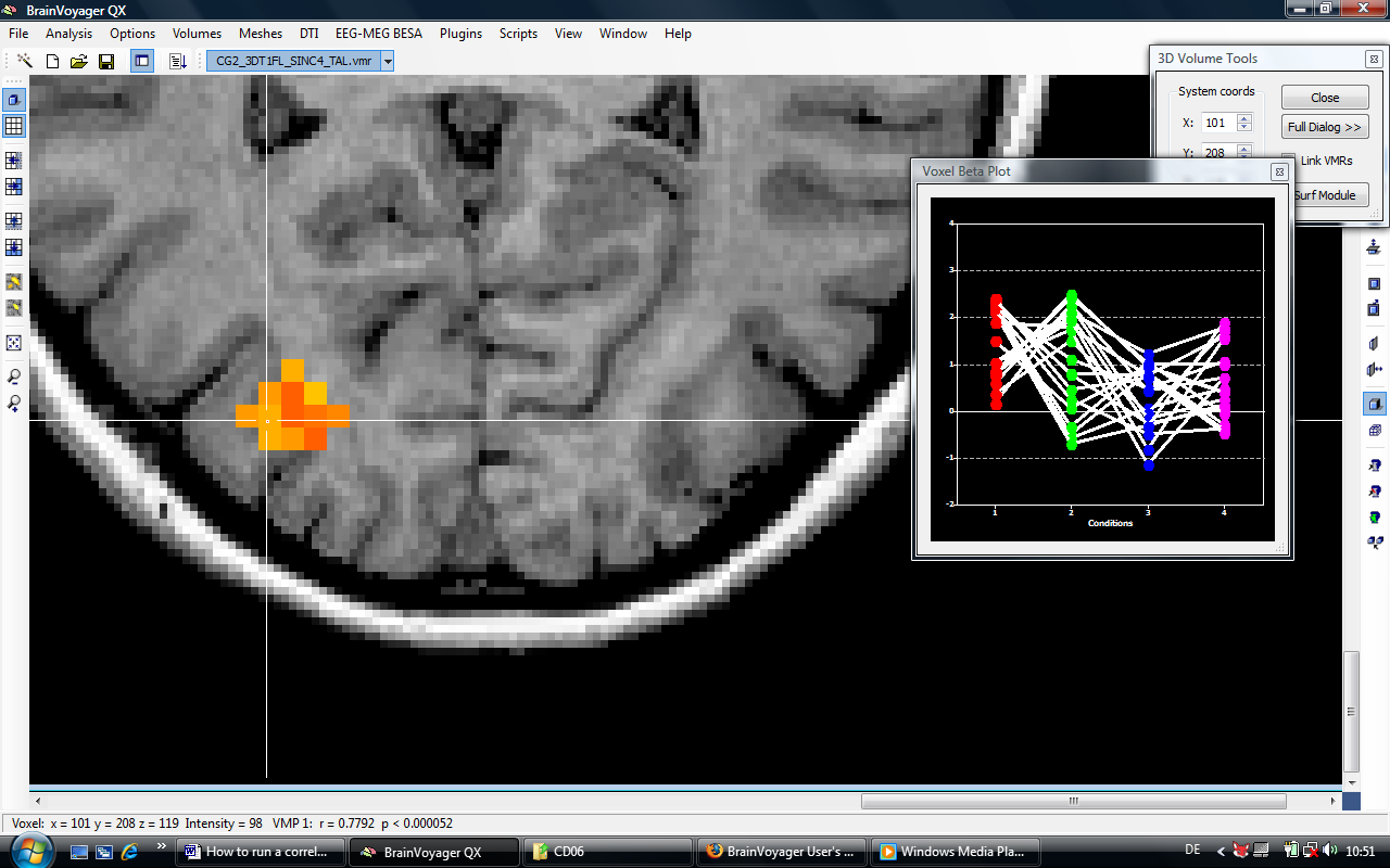
3. We choose the voxel currently selecting by the crosshair (X: 101, Y:208, Z:119) and hold down the “Shift” button to deactivate the automatic refresh of voxel values while moving the mouse.
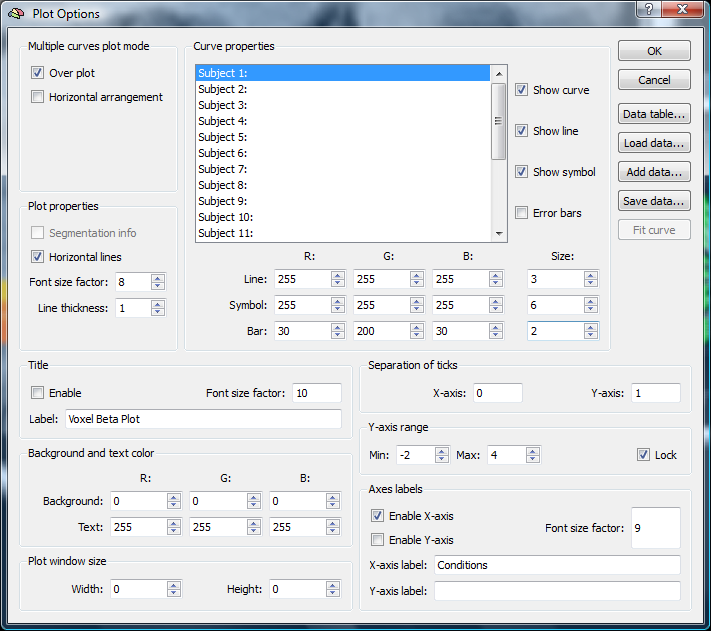
4. When clicking in the plot, we have several options, e.g. to save the voxel values.
We save the beta values as a “dat” file clicking the “Save data” button.
Now we are ready to analyze the data externally. We use Excel for this purpose.
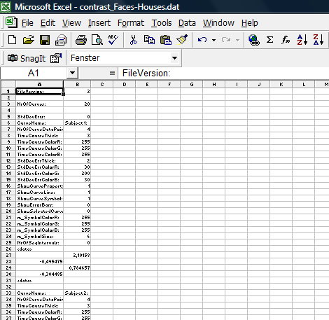
5. After importing the dat file into Excel, we can see that the file structure is possibly not optimal to run external calculation. For each plot (there is one for each of the 20 Subjects), there is a small header we have to get rid of.
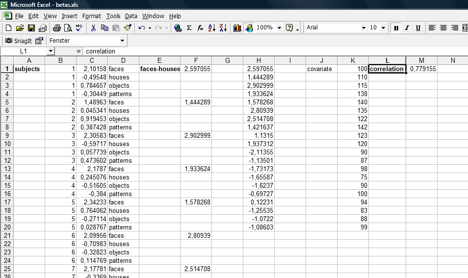
In Excel, we reorganize the data in a way that allows an easy calculation of the correlation between the contrast value and the covariate (pseudo-IQ). We basically concatenate all the beta values of all subject, generate a new column subtracting the condition betas from each other (nothing more than redoing the contrast without taking the standard error into account), enter the covariate values in a new column and finally run the correlation (this is defined as a standard function in Excel). The covariate values can be imported from the .cov file saved before. Because the reformatting is a quite tedious and repetetive affair, one could write an Excel macro that performs this step automatically. More details can be obtained from the author.
The following screenshot shows the data after reorganisation. The value of the correlation can be seen in cell M1. The value (0.779155) is exactly the same (given some rounding of decimals) as provided by BV.